Page 43 - Advanced thermodynamics for engineers

26 CHAPTER 2 THE SECOND LAW AND EQUILIBRIUM

2.12 GIBBS ENERGY AND PHASES
An extremely important feature of Gibbs energy is that it defines the interaction of coexisting phases
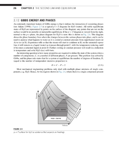
(see Atkins (1994)). Figure 2.5 is a typical p–v–T diagram for H 2 O (water). All stable equilibrium
states of H 2 O are represented by points on the surface of the diagram: any points that are not on the
surface would be in unstable or metastable equilibrium. If the p–v–T diagram is viewed from the right,
normal to the p–v plane, the phase diagram for H 2 O is seen: this is shown in Fig. 2.6. This diagram
shows the phase boundary lines where the changes between the various phases take place, and it can be
used to analyse what happens to water as it is cooled at constant pressure from superheated steam (at
A) to ice (at E). Experience tells us that the steam will start to condense at B, on the saturated vapour
line; it will remain as a liquid (water) as it passes through point C, with the temperature reducing, until
it becomes a saturated liquid at point D. Further cooling at constant pressure will result in a reduction
in temperature and solid H 2 O (ice) will form.
An interesting question is how many properties are required to define the state of the system when a
number of components, C, in a number of different phases, P, are present. This problem was solved by
Gibbs, and his phase rule states that for a system at equilibrium the number of degrees of freedom, D,
(equal to the number of independent intensive properties) is
D ¼ C P þ 2 (2.31)
Most mechanical engineering problems only deal with multiple phase mixtures of single com-
ponents, e.g. H 2 O. Hence, for the regions shown in Fig. 2.6, where there is a single component present

Pressure liquid gas Critical

point

solid liquid + vapour
Temperature
Triple point
solid + vapour

Volume
FIGURE 2.5
p–v–T surface for H 2 O (a substance that expands on freezing).