Page 133 - Advanced Mine Ventilation

114 Advanced Mine Ventilation

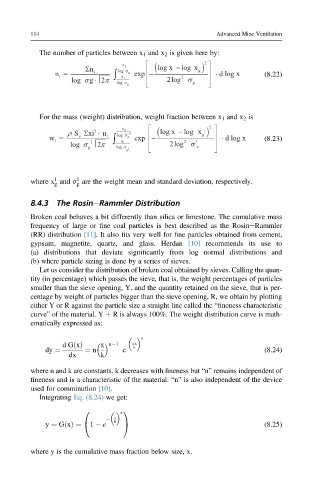
The number of particles between x 1 and x 2 is given here by:
x
Σ n log σ ⎡ ( log x g )log x − 2 ⎤
n= i x ∫ exp ⎢ ⎥ − ⋅ d log x (8.22)
i
log σ g⋅ 2π log σ ⎢ ⎣ 2log σ g ⎥ ⎦
2

For the mass (weight) distribution, weight fraction between x 1 and x 2 is
x ⎡ ( 2 ⎤
ρ S Σ xi ⋅ 3 n log σ log x ) log x −
⎢
w= v i x ∫ exp − ⎥ ∙ d log x (8.23)
i
log σ 1 2π ⎢ 2log σ 1 ⎥
2
g log σ ⎣ ⎦
1
1
where x and s are the weight mean and standard deviation, respectively.
g g
8.4.3 The RosineRammler Distribution
Broken coal behaves a bit differently than silica or limestone. The cumulative mass
frequency of large or fine coal particles is best described as the RosineRammler
(RR) distribution [11]. It also fits very well for fine particles obtained from cement,
gypsum, magnetite, quartz, and glass. Herdan [10] recommends its use to
(a) distributions that deviate significantly from log normal distributions and
(b) where particle sizing is done by a series of sieves.
Let us consider the distribution of broken coal obtained by sieves. Calling the quan-
tity (in percentage) which passes the sieve, that is, the weight percentages of particles
smaller than the sieve opening, Y, and the quantity retained on the sieve, that is per-
centage by weight of particles bigger than the sieve opening, R, we obtain by plotting
either Y or R against the particle size a straight line called the “fineness characteristic
curve” of the material. Y þ R is always 100%. The weight distribution curve is math-
ematically expressed as:

n
x n 1
dGðxÞ x
k
dy ¼ ¼ n e (8.24)
dx k
where n and k are constants. k decreases with fineness but “n” remains independent of
fineness and is a characteristic of the material. “n” is also independent of the device
used for comminution [10].
Integrating Eq. (8.24) we get:

0 n 1
x
k
y ¼ GðxÞ¼ @ 1 e A (8.25)

where y is the cumulative mass fraction below size, x.