Page 225 - Advances in Biomechanics and Tissue Regeneration

11.2 METHODOLOGY OF SIMULATION 221

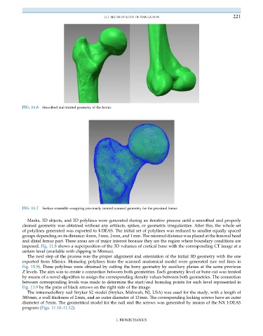
FIG. 11.6 Smoothed and treated geometry of the femur.

FIG. 11.7 Surface ensemble wrapping previously treated scanned geometry for the proximal femur.

Masks, 3D objects, and 3D polylines were generated during an iterative process until a smoothed and properly
cleaned geometry was obtained without any artifacts, spikes, or geometric irregularities. After this, the whole set
of polylines generated was exported to I-DEAS. The initial set of polylines was reduced to smaller equally spaced
groups depending on its distance: 4mm, 3mm, 2mm, and 1mm. The minimal distance was placed at the femoral head
and distal femur part. These areas are of major interest because they are the region where boundary conditions are
imposed. Fig. 11.8 shows a superposition of the 3D volumes of cortical bone with the corresponding CT image at a
certain level (available with clipping in Mimics).
The next step of the process was the proper alignment and orientation of the initial 3D geometry with the one
exported from Mimics. Homolog polylines from the scanned anatomical model were generated (see red lines in
Fig. 11.9). These polylines were obtained by cutting the bony geometry by auxiliary planes at the same previous
Z levels. The aim was to create a connection between both geometries. Each geometry level or bone cut was treated
by means of a novel algorithm to assign the corresponding density values between both geometries. The connection
between corresponding levels was made to determine the start/end homolog points for each level represented in
Fig. 11.9 by the pairs of black arrows on the right side of the image.
The intramedullary nail Stryker S2 model (Stryker, Mahwah, NJ, USA) was used for the study, with a length of
380mm, a wall thickness of 2mm, and an outer diameter of 13mm. The corresponding locking screws have an outer
diameter of 5mm. The geometrical model for the nail and the screws was generated by means of the NX I-DEAS
program (Figs. 11.10–11.12).

I. BIOMECHANICS