Page 334 - Advances in Biomechanics and Tissue Regeneration

332 16. ON THE SIMULATION OF ORGAN-ON-CHIP CELL PROCESSES

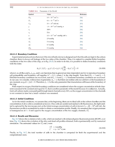
TABLE 16.1 Parameters of the Model
Symbol Value Reference
2
1.0 10 5 cm /s [56]
D O 2
2
D n 6.6 10 12 cm /s [54]
7
C sat 3.5 10 cell/mL [57]
2
χ 1.5 10 9 cm /mmHg s [58]
τ n 300 h [58]
τ d 72 h [59]
3
α 1.0 10 9 cm mmHg/cell s [60]
O K 2.5 mmHg [56]
2
O ∗ 2 7.0 mmHg [54]

O d 2 0.7 mmHg [54]
δO 2 0.1 mmHg [54]

16.6.1.2 Boundary Conditions
Experimental practice shows that even if the microfluidic device is designed such that the cells are kept in the culture
chamber, there is always cell leakage at the two sides of the chamber. Thus, it is natural to consider Robin boundary
conditions at the two sides of the chip, as in Eq. (16.3). In order to do this, it is possible to define boundary conditions
with the form:

∗ ∗ ∗ ∂f n ∗
h n ðx ,tÞ ¼ 0 (16.109)
∂x
K n ðx ,tÞðC n g n ðx ,tÞÞ + J n ðx ,tÞ
where f n is cell flux and k n , J n , g n , and f n are functions that in general are time-dependent and try to reproduce boundary
cell permeability and boundary cell supplies (x* ¼ 0, L, where L is the chip length). Note that if K n ¼ 1 and J n ¼ 0,
Dirichlet boundary conditions are recovered, and if K n ¼ 0 and J n ¼ 1, Neumann boundary conditions are recovered.
In our case, we consider, without loss of generality, K n ¼ 1, that there are neither cells nor cell flow at the boundaries at
any moment, so g n (t) ¼ f n (t) ¼ 0. Therefore, J n ¼ J is the only parameter that characterizes cell losses at the boundary of
the chip.
With respect to oxygen, Dirichlet boundary conditions are considered where the oxygen concentration at both chan-
S
nels is assumed to be constant and equal to O , that is another parameter of the model because it is unknown. Actually,
2
fresh cell culture media were perfused through lateral channels every 24 h, so the oxygen concentration in the channels
is not constant in time but a small variation was assumed.

16.6.1.3 Initial Conditions
As for the initial conditions, we assume that, at the beginning, there are no dead cells at the culture chamber and the
concentration of alive cells is considered as known. Once cells are seeded and marked with fluorescence, the light emit-
6
ted is captured by the microscope and, as the initial average concentration of cells is known C 0 ¼ 40 10 cell/mL, the
fluorescence profile is normalized in order to obtain a concentration profile. Finally, it is assumed that oxygen pressure
S
is homogeneous at t ¼ 0 and equal to the oxygen concentration at the two supply channels, O .
2
16.6.1.4 Results and Discussion
Fig. 16.5 shows the evolution of alive cells, which are marked with enhanced green fluorescent protein (EGFP), over
time. Fig. 16.6 shows the evolution of the alive and dead cell profiles obtained, both experimentally and by numerical
S
simulation. The estimated values for O and J were
2
O S ¼ 7 mmHg
2 (16.110)
16
J ¼ 5 10 s=cm
Finally, in Fig. 16.7, the total number of cells in the chamber is computed for both the experimental and the
computational cases.

II. MECHANOBIOLOGY AND TISSUE REGENERATION