Page 146 - Advances in Renewable Energies and Power Technologies

1. Introduction 119

Start

Sense V, I

P(i) =V(i)*I(i)

Yes
P(i)-P(i-1) =0
No
No Yes
P(i)-P(i-1) >0
Yes No No Yes
U(i)-U(i-1) >0 V(i)-V(i-1) >0

V(i)=V(i)-Δ V(i) =V(i)+Δ V(i) =V(i)-Δ V(i) =V(i)+Δ

return

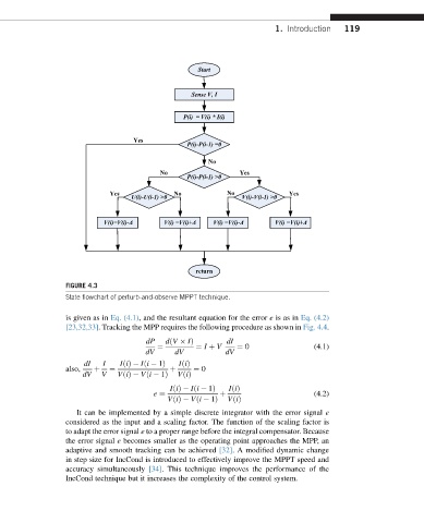
FIGURE 4.3
State flowchart of perturb-and-observe MPPT technique.

is given as in Eq. (4.1), and the resultant equation for the error e is as in Eq. (4.2)
[23,32,33]. Tracking the MPP requires the following procedure as shown in Fig. 4.4.
dP dðV IÞ dI
¼ ¼ I þ V ¼ 0 (4.1)
dV dV dV
dI I IðiÞ Iði 1Þ IðiÞ
also, þ ¼ þ ¼ 0
dV V VðiÞ Vði 1Þ VðiÞ

IðiÞ Iði 1Þ IðiÞ
e ¼ þ (4.2)
VðiÞ Vði 1Þ VðiÞ
It can be implemented by a simple discrete integrator with the error signal e
considered as the input and a scaling factor. The function of the scaling factor is
to adapt the error signal e to a proper range before the integral compensator. Because
the error signal e becomes smaller as the operating point approaches the MPP, an
adaptive and smooth tracking can be achieved [32]. A modified dynamic change
in step size for IncCond is introduced to effectively improve the MPPT speed and
accuracy simultaneously [34]. This technique improves the performance of the
IncCond technique but it increases the complexity of the control system.