Page 114 - Aerodynamics for Engineering Students

Governing equations of fluid mechanics 97

h

Y A

X -
......................................... V
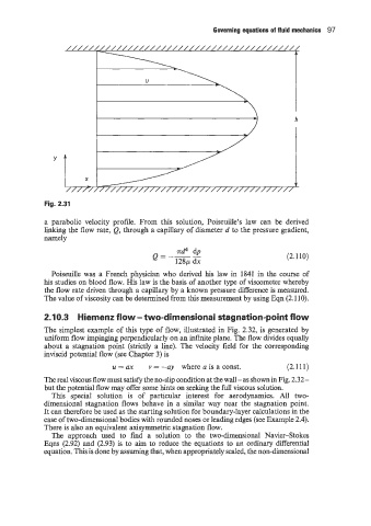
Fig. 2.31

a parabolic velocity profile. From this solution, Poiseuille’s law can be derived
linking the flow rate, Q, through a capillary of diameter d to the pressure gradient,
namely
Q=--- 7rd4 dp (2.110)
128p dx

Poiseuille was a French physician who derived his law in 1841 in the course of
his studies on blood flow. His law is the basis of another type of viscometer whereby
the flow rate driven through a capillary by a known pressure difference is measured.
The value of viscosity can be determined from this measurement by using Eqn (2.110).

2.10.3 Hiemenz flow - two-dimensional stagnation-point flow
The simplest example of this type of flow, illustrated in Fig. 2.32, is generated by
uniform flow impinging perpendicularly on an infinite plane. The flow divides equally
about a stagnation point (strictly a line). The velocity field for the corresponding
inviscid potential flow (see Chapter 3) is
u = ax v = -ay where a is a const. (2.111)

The real viscous flow must satisfy the no-slip condition at the wall - as shown in Fig. 2.32 -
but the potential flow may offer some hints on seeking the full viscous solution.
This special solution is of particular interest for aerodynamics. All two-
dimensional stagnation flows behave in a similar way near the stagnation point.
It can therefore be used as the starting solution for boundary-layer calculations in the
case of two-dimensional bodies with rounded noses or leading edges (see Example 2.4).
There is also an equivalent axisymmetric stagnation flow.
The approach used to find a solution to the two-dimensional Navier-Stokes
Eqns (2.92) and (2.93) is to aim to reduce the equations to an ordinary differential
equation. This is done by assuming that, when appropriately scaled, the non-dimensional