Page 53 - Aeronautical Engineer Data Book

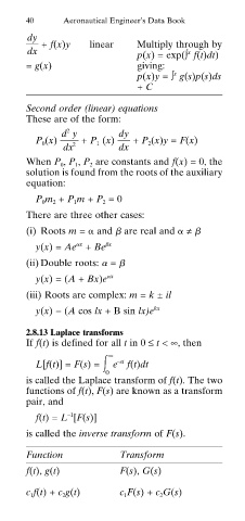
40 Aeronautical Engineer’s Data Book
dy
33 + f(x)y linear Multiply through by
dx x
p(x) = exp(∫ f(t)dt)
= g(x) giving:
x
p(x)y = ∫ g(s)p(s)ds
+ C

Second order (linear) equations
These are of the form:
2
d y dy
P 0 (x) 33 + P 1 (x) 33 + P 2 (x)y = F(x)
dx 2 dx
When P , P 1 , P 2 are constants and f(x) = 0, the
0
solution is found from the roots of the auxiliary
equation:
P 0 m 2 + P 1 m + P 2 = 0
There are three other cases:
(i) Roots m = and are real and ≠
x
y(x) = Ae + Be x
(ii) Double roots: =

y(x) = (A + Bx)e x
(iii) Roots are complex: m = k ± il
y(x) = (A cos lx + B sin lx)e kx
2.8.13 Laplace transforms
If f(t) is defined for all t in 0 ≤ t < ∞, then
∞
–st
L[f(t)] = F(s) = � e f(t)dt
0
is called the Laplace transform of f(t). The two
functions of f(t), F(s) are known as a transform
pair, and
–1
f(t) = L [F(s)]
is called the inverse transform of F(s).
Function Transform
f(t), g(t) F(s), G(s)

c 1 f(t) + c 2 g(t) c 1 F(s) + c 2 G(s)