Page 363 - Air pollution and greenhouse gases from basic concepts to engineering applications for air emission control

11.3 Gaussian-Plume Dispersion Models 341

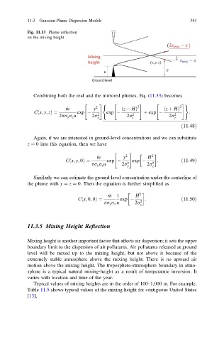
Fig. 11.13 Plume reflection
on the mixing height

Combining both the real and the mirrored plumes, Eq. (11.33) becomes

" #( " 2 # " 2 #)
_ m y 2 ð z HÞ ð z þ HÞ
Cx; y; zÞ ¼ exp 2 exp 2 þ exp 2 :
ð
2pr y r z u 2r 2r 2r
y z z
ð11:48Þ
Again, if we are interested in ground-level concentrations and we can substitute
z ¼ 0 into this equation, then we have

" #
_ m y 2 H 2
ð
Cx; y; 0Þ ¼ exp exp : ð11:49Þ
pr y r z u 2r 2 y 2r 2 z
Similarly we can estimate the ground-level concentration under the centerline of
the plume with y ¼ z ¼ 0. Then the equation is further simplified as

_ m 1 H 2
Cx; 0; 0Þ ¼ exp : ð11:50Þ
ð
pr y r z u 2r 2 z

11.3.5 Mixing Height Reflection

Mixing height is another important factor that affects air dispersion; it sets the upper
boundary limit to the dispersion of air pollutants. Air pollutants released at ground
level will be mixed up to the mixing height, but not above it because of the
extremely stable atmosphere above the mixing height. There is no upward air
motion above the mixing height. The troposphere-stratosphere boundary in atmo-
sphere is a typical natural mixing-height as a result of temperature inversion. It
varies with location and time of the year.
Typical values of mixing heights are in the order of 100–1,000 m. For example,
Table 11.5 shows typical values of the mixing height for contiguous United States
[13].