Page 359 - Air pollution and greenhouse gases from basic concepts to engineering applications for air emission control

11.3 Gaussian-Plume Dispersion Models 337

In reality, the plume rise stops at certain height, and the maximum plume rise is
achieved at a critical distance of x c . The critical distance can be estimated using
(
5=8 4 3
49F for F B \55 m =s
x c ¼ B 2=5 ð11:42Þ
4
119F for F B [ 55 m =s 3
B
And the corresponding maximum plume rise is
8
3=4
F 4 3
21:4 u for F B \55 m =s
< B
Dh m ffi ð11:43Þ
F 3=5
38:7 for F B [ 55 m =s
: B 4 3
u
In Example 11.3, we used the maximum plume rise for calculation. The actual
ground-level concentration can now be predicted with improved accuracy if we
consider the local plume rise.
Example 11.4: Plume rise
Consider a power plant stack with a diameter of d s ¼ 1:2 m and the stack emission
gas is discharged at the speed of v s ¼ 5m=s. Assume horizontal wind speed
u ¼ 1:1m=s, and surrounding air temperature is T a ¼ 300 K. Plot the plume rise
downwind the emission source for discharge temperature of T s ¼ 500 K.
Solution
Since the from a power plant is buoyancy-dominant plume, we only consider the
buoyancy flux

2 2
T a d 300 1:2 4 3
F B ¼ 1 s gv s ¼ 1 9:81 1:1 ¼ 7:063 m =s
T s 4 500 2

4
3
Since F B \ 55 m =s the corresponding maximum plume rise is calculated using
21:4 3=4
Dh m ¼ F B ¼ 84:3m
u

For T e ¼ 500 K, the transitional plume rise can then be determined using
1 1

3 25 7:063 3
25 F B 2 2
Dh ¼ 3 x ¼ 3 x
6 u 6 1:1
2 1=3

¼ 22:11x
2 1=3
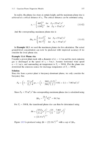
Figure 11.9 is produced using Dh ¼ 22:11x Þ with a cap of Dh m .
ð