Page 355 - Air pollution and greenhouse gases from basic concepts to engineering applications for air emission control

11.3 Gaussian-Plume Dispersion Models 333

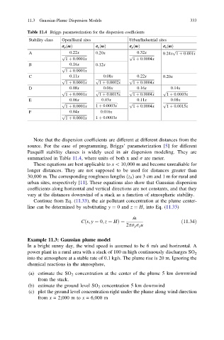
Table 11.4 Briggs parameterization for the dispersion coefficients
Stability class Open/Rural sites Urban/Industrial sites
r y ðmÞ r z mðÞ r y ðmÞ r z ðmÞ
p
A 0:22x 0:20x 0:32x 0:24x 1 þ 0:001x
ffiffiffiffiffiffiffiffiffiffiffiffiffiffiffiffiffiffiffiffiffiffi
p ffiffiffiffiffiffiffiffiffiffiffiffiffiffiffiffiffiffiffiffiffiffiffiffi p ffiffiffiffiffiffiffiffiffiffiffiffiffiffiffiffiffiffiffiffiffiffiffiffi
1 þ 0:0001x 1 þ 0:0004x
B 0:16x 0:12x
p ffiffiffiffiffiffiffiffiffiffiffiffiffiffiffiffiffiffiffiffiffiffiffiffi
1 þ 0:0001x
C 0:11x 0:08x 0:22x 0:20x
p ffiffiffiffiffiffiffiffiffiffiffiffiffiffiffiffiffiffiffiffiffiffiffiffi p ffiffiffiffiffiffiffiffiffiffiffiffiffiffiffiffiffiffiffiffiffiffiffiffi p ffiffiffiffiffiffiffiffiffiffiffiffiffiffiffiffiffiffiffiffiffiffiffiffi
1 þ 0:0001x 1 þ 0:0002x 1 þ 0:0004x
D 0:08x 0:06x 0:16x 0:14x
p ffiffiffiffiffiffiffiffiffiffiffiffiffiffiffiffiffiffiffiffiffiffiffiffi p ffiffiffiffiffiffiffiffiffiffiffiffiffiffiffiffiffiffiffiffiffiffiffiffi p ffiffiffiffiffiffiffiffiffiffiffiffiffiffiffiffiffiffiffiffiffiffiffiffi p ffiffiffiffiffiffiffiffiffiffiffiffiffiffiffiffiffiffiffiffiffiffiffiffi
1 þ 0:0001x 1 þ 0:0015x 1 þ 0:0004x 1 þ 0:0003x
E 0:06x 0:03x 0:11x 0:08x
p ffiffiffiffiffiffiffiffiffiffiffiffiffiffiffiffiffiffiffiffiffiffiffiffi . p ffiffiffiffiffiffiffiffiffiffiffiffiffiffiffiffiffiffiffiffiffiffiffiffi p ffiffiffiffiffiffiffiffiffiffiffiffiffiffiffiffiffiffiffiffiffiffiffiffi
1 þ 0:0001x 1 þ 0:0003x 1 þ 0:0004x 1 þ 0:0015x
F 0:04x 0:016x
p ffiffiffiffiffiffiffiffiffiffiffiffiffiffiffiffiffiffiffiffiffiffiffiffi
1 þ 0:0001x 1 þ 0:0003x

Note that the dispersion coefficients are different at different distances from the
source. For the ease of programming, Briggs’ parameterization [5] for different
Pasquill stability classes is widely used in air dispersion modeling. They are
summarized in Table 11.4, where units of both x and r are meter.
These equations are best applicable to x \ 10;000 m and become unrealiable for
longer distances. They are not supposed to be used for distances greater than
30;000 m. The corresponding roughness lengths ðz 0 Þ are 3 cm and 1 m for rural and
urban sites, respectively [11]. These equations also show that Gaussian dispersion
coefficients along horizontal and vertical directions are not constants, and that they
vary at the distances downwind of a stack as a function of atmospheric stability.
Continue from Eq. (11.33), the air pollutant concentration at the plume center-
line can be determined by substituting y ¼ 0 and z ¼ H, into Eq. (11.33)

_ m
Cx; y ¼ 0; z ¼ HÞ ¼ ð11:34Þ
ð
2pr y r z u
Example 11.3: Gaussian plume model
In a bright sunny day, the wind speed is assumed to be 6 m/s and horizontal. A
power plant in a rural area with a stack of 100 m high continuously discharges SO 2
into the atmosphere at a stable rate of 0.1 kg/s. The plume rise is 20 m. Ignoring the
chemical reactions in the atmosphere,
(a) estimate the SO 2 concentration at the center of the plume 5 km downwind
from the stack.
(b) estimate the ground level SO 2 concentration 5 km downwind
(c) plot the ground level concentration right under the plume along wind direction
from x = 2,000 m to x = 6,000 m