Page 353 - Air pollution and greenhouse gases from basic concepts to engineering applications for air emission control

11.3 Gaussian-Plume Dispersion Models 331

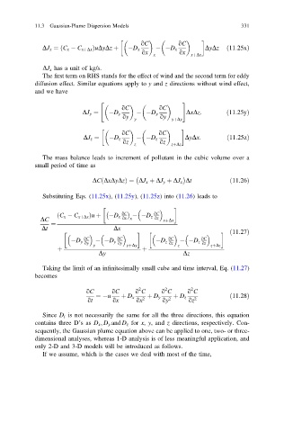
oC oC

DJ x ¼ C x C xþDx ÞuDyDz þ D x D x DyDz ð11:25xÞ
ð
ox ox
x xþDx
DJ x has a unit of kg/s.
The first term on RHS stands for the effect of wind and the second term for eddy
diffusion effect. Similar equations apply to y and z directions without wind effect,
and we have

" #

oC oC
DJ y ¼ D y D y DxDz: ð11:25yÞ
oy oy
y yþDy
oC oC

DJ z ¼ D z D z DyDx: ð11:25zÞ
oz oz
z zþDz
The mass balance leads to increment of pollutant in the cubic volume over a
small period of time as

DC DxDyDzÞ ¼ DJ x þ DJ y þ DJ x Dt ð11:26Þ
ð
Substituting Eqs. (11.25x), (11.25y), (11.25z) into (11.26) leads to

oC oC
ð C x C xþDx Þu þ D x ox x D z oz
DC xþDx
¼
Dt Dx
ð11:27Þ

oC oC oC oC
D y oy D y oy D z oz D z oz
y yþDy z zþDz
þ þ
Dy Dz
Taking the limit of an infinitesimally small cube and time interval, Eq. (11.27)
becomes
2 2 2
oC oC o C o C o C
¼ u þ D x þ D y þ D z ð11:28Þ
ot ox ox 2 oy 2 oz 2
Since D i is not necessarily the same for all the three directions, this equation
contains three D’sas D x ; D y and D z for x, y,and z directions, respectively. Con-
sequently, the Gaussian plume equation above can be applied to one, two- or three-
dimensional analyses, whereas 1-D analysis is of less meaningful application, and
only 2-D and 3-D models will be introduced as follows.
If we assume, which is the cases we deal with most of the time,