Page 351 - Air pollution and greenhouse gases from basic concepts to engineering applications for air emission control

11.2 General Gaussian Dispersion Model 329

( " # )
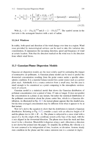
2 2

u 1 z 1 b þ 1 b þ 1Þ
ð
0
0
¼ ln þ ln þ 2 arctan bðÞ arctan b ðÞ½ 0 Š :
k k 2 2
ð
u z 0 b þ 1 b þ 1Þ
|fflfflfflfflfflfflfflfflfflfflfflfflfflfflfflfflfflfflfflfflfflfflfflfflfflfflfflfflfflfflfflfflfflfflfflfflfflfflfflfflfflfflfflfflfflfflfflfflfflffl{zfflfflfflfflfflfflfflfflfflfflfflfflfflfflfflfflfflfflfflfflfflfflfflfflfflfflfflfflfflfflfflfflfflfflfflfflfflfflfflfflfflfflfflfflfflfflfflfflfflffl}
ð11:23Þ
0:25 0:25
ð
With b ¼ 1 15z 0 =Lð Þ and b ¼ 1 15z=LÞ . The symbol arctan in the
0
last term is the arctangent function with a unit of radian.
11.2.6.4 Windrose
In reality, both speed and direction of the wind change over time in a region. Wind
roses provided by meteorological services can be used to take this variation into
consideration. It summarizes the incoming direction, speed and frequency of wind
at certain location. Note that the direction marked on the wind rose is the direction
from which wind blows.

11.3 Gaussian-Plume Dispersion Models

Gaussian air dispersion models are the most widely used for estimating the impact
of nonreactive air pollutants. A Gaussian-plume model can be used to predict the
downwind concentration resulting from the point source under a specific atmo-
spheric condition. It is a material balance model for a point source such as a power
plant stack. Admittedly it is a source emission from a small area, but this area is
small enough to be considered as a point comparing to the atmospheric environ-
ment of concern.
Gaussian model is a statistical model that shows the Gaussian distribution of
pollutant concentration over a period of time, 15 min or longer. It does not predict
the concentration in a plume at any instant, but rather the statistical distribution of
the pollutant concentration about the plume center line, which is a Gaussian dis-
tribution. As illustrated in Fig. 11.7, the instant plume appears like the shaded area,
but the time-averaged concentration may be different from what it appears to be at
that instant.
Now let’s derive the equation to show that the distribution is indeed a Gaussian
distribution. Referring to Fig. 11.7, consider a stack with an effective height of H
and the plume rise is (Dh ¼ H h). The plume is subjected to a cross wind with a
speed of u. Set the origin of the coordinate system at the base of the stack, with the
x axis aligned in the downwind direction. The plume rises from the stack and then
travel in the x direction. Meanwhile it disperses along y and z directions.y direction
is not shown but pointed into the paper. To simplify the problem, the velocity u is
for now assumed to be independent of time, location, or elevation. Assume steady
state condition in the plume and the source emission rate is a constant _ m (kg/s).