Page 364 - Air pollution and greenhouse gases from basic concepts to engineering applications for air emission control

342 11 Air Dispersion

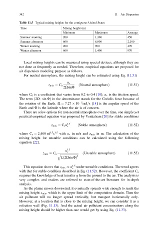
Table 11.5 Typical mixing heights for the contiguous United States
Time Mixing height (m)
Minimum Maximum Average
Summer morning 200 1,100 450
Summer afternoon 600 4,000 2,100
Winter morning 200 900 470
Winter afternoon 600 1,400 970

Local mixing heights can be measured using special devices, although they are
not done as frequently as needed. Therefore, empirical equations are proposed for
air dispersion modeling purpose as follows.
For neutral atmosphere, the mixing height can be estimated using Eq. (11.51)

u
z mix ¼ C 0 ðNeutral atmosphereÞ ð11:51Þ
2XsinU
where C 0 is a coefficient that varies from 0.2 to 0.4 [10]; u is the friction speed.
The term 2X sin UÞ in the denominator stands for the Coriolis force because of
ð
5
the rotation of the Earth. X ¼ 7:27 10 rad=s[18] is the angular speed of the
Earth and U is the latitude where the air is of concern.
There are a few options for non-neutral atmosphere over the time, one simple yet
practical empirical equation was proposed by Venkatram [20] for stable conditions

z mix ¼ C s u 1:5 ðStable atmosphereÞ ð11:52Þ

0:5 1:5
where C s ¼ 2;400 m s with u in m/s and z mix in m. The calculation of the
mixing height for unstable conditions can be calculated using the following
equation [22].

u 1:5
ðUnstable atmosphere) ð11:53Þ
z mix ¼ C u q ffiffiffiffiffiffiffiffiffiffiffiffiffiffiffiffiffiffiffiffiffiffiffiffi
3
ð
L 2XsinUÞ
This equation shows that z mix / u 1:5 under unstable conditions. The trend agrees

with that for stable condition described in Eq. (11.52). However, the coefficient C u
requires the knowledge of heat transfer q from the ground to the air. The analysis is
very complex and readers are referred to state-of-the-art literature for in-depth
analysis.
As the plume moves downwind, it eventually spreads wide enough to reach the
mixing height z mix , which is the upper limit of the computation domain. Then the
air pollutant will no longer spread vertically, but transport horizontally only.
However, at a location that is close to the mixing height, we can consider it as a
refection wall (Fig. 11.13). And the actual air pollutant concentrations along the
mixing height should be higher than one would get by using Eq. (11.33).