Page 31 - Algorithm Collections for Digital Signal Processing Applications using MATLAB

1. Artificial Intelligence 19

selecting the values corresponding to higher energy levels are more. This
process of selecting the values randomly is repeated for the finite number of
iteration. The values obtained after the finite number of iteration can be
assumed as the values with lowest energy state (i.e) lowest cost function
Thus the simulated Annealing algorithm is summarized as follow.

3.1 Simulated Annealing Algorithm

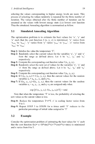
The optimization problem is to estimate the best values for ‘x’, ‘y’ and
‘z’ such that the cost function f (x, y, z) is minimized. ‘x’ varies from
‘x min ‘to ‘x max’. ‘y’ varies from ‘y’ varies ‘y min’ to ‘y max’ .’z’ varies from
‘z min’ to ‘z max’

Step 1: Intialize the value the temperature ‘T’.
Step 2: Randomly select the current values for the variables ‘x’, ’y’ and ‘z’
from the range as defined above. Let it be ‘x c ’, ‘y c’ and ‘z c ’
respectively.
Step 3: Compute the corresponding cost function value f (x c, y c, z c).
Step 4: Randomly select the next set of values for the variables ‘x’, ’y’ and
‘z’ from the range as defined above. Let it be ‘x n ’, ‘y n’ and ‘z n’
respectively.
Step 5: Compute the corresponding cost function value f (x n, y n, z n).
Step 6: If f (x n, y n, z n)<= f (x c, y c, z c), then the current values for the random
variables x c = x n, y c,= y n and z c=z . n
Step 7: If f(x n, y n, z n)>f(x c, y c, z c), then the current values for the random
variables x c = x n, y c,= y n and z c=z n are assigned only when

exp [(f (x c, y c, z c)- f(x n, y n, z n))/T] > rand

Note that when the temperature ‘T’ is less, the probability of selecting the
new values as the current values is less.

Step 8: Reduce the temperature T=r*T. r’ is scaling factor varies from
0 to 1.
Step 9: Repeat STEP 3 to STEP8 for n times until ‘T’ reduces to the
particular percentage of initial value assigned to ‘T’

3.2 Example

Consider the optimization problem of estimating the best values for ‘x’ such
that the cost function f(x)= x+10*sin(5*x)+7*cos(4*x)+sin(x) is minimized
and x varies from 0 to 5.