Page 32 - Algorithm Collections for Digital Signal Processing Applications using MATLAB

20 Chapter 1

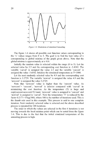
Figure 1-6 Illustration of simulated Annealing

The figure 1-6 shows all possible cost function values corresponding to
the ‘x’ values ranges from 0 to 5. The goal is to find the best value of x
corresponding to global minima of the graph given above. Note that the
global minima is approximately at x=0.8.
Initially the random value is selected within the range (0 to 5). Let the
selected value be 2.5 and the corresponding cost function is -3.4382. The
variable ‘curval’ is assigned the value 2.5 and the variable ‘curcost’ is
assigned the value -3.4382. Intialize the simulated temperature as T=1000.
Let the next randomly selected value be 4.9 and the corresponding cost
function is 3.2729. The variable ‘newval’ is assigned the value 4.9 and the
‘newcost’ is assigned the value 3.2729.
Note that ‘newcost’ value is higher than the ‘curcost’ value. As
‘newcost’> ‘curcost’, ‘newval’ is inferior compared with ‘curval’ in
minimizing the cost function. As the temperature (T) is large and
exp((curcost-newcost)/T)>rand, ‘newcost’ value is assigned to ‘curcost’ and
‘newval’ is assigned to ‘curval’. Now the temperature ‘T’ is reduced by the
factor 0.2171=1/log(100), where 100 is the number of iterations used. This is
the thumb rule used in this example. This process is said to one complete
iteration. Next randomly selected value is selected and the above described
process is repeated for 100 iterations.
The order in which the values are selected in the first 6 iterations is not
moving towards the local minima point which can be noted from the figure
1-6. This is due to the fact that the initial simulated temperature of the
annealing process is high.