Page 36 - Algorithm Collections for Digital Signal Processing Applications using MATLAB

24 Chapter 1

4. BACK PROPAGATION NEURAL NETWORK

The mathematical model of the Biological Neural Network is defined as
Artificial Neural Network. One of the Neural Network models which are
used almost in all the fields is Back propagation Neural Network.
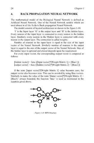
The model consists of layered architecture as shown in the figure 1-10.
‘I’ is the Input layer ‘O’ is the output layer and ‘H’ is the hidden layer.
Every neuron of the input layer is connected to every neuron in the hidden
layer. Similarly every neuron in the Hidden layer is connected with every
neuron in the output layer. The connection is called weights.
Number of neurons in the input layer is equal to the size of the input
vector of the Neural Network. Similarly number of neurons in the output
layer is equal to the size of the output vector of the Neural Network. Size of
the hidden layer is optional and altered depends upon the requirement
For every input vector, the corresponding output vector is computed as
follows

[hidden vector] = func ([Input vector]*[Weight Matrix 1] + [Bias1 ])
[output vector] = func ([hidden vector]*[Weight Matrix 2] + [Bias2 ])

If the term [Input vector]*[Weight Matrix 1] value becomes zero, the
output vector also becomes zero. This can be avoided by using Bias vectors.
Similarly to make the value of the term ‘[Input vector]*[Weight Matrix 1] +

[Bias1]’ always bounded, the function ‘func’ is used as mentioned in the
equation given above.

Figure 1-10 BPN Structure