Page 40 - Algorithm Collections for Digital Signal Processing Applications using MATLAB

28 Chapter 1

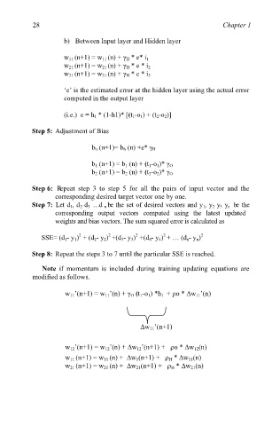
b) Between Input layer and Hidden layer

w 11 (n+1) = w 11 (n) + γ H * e* i 1
w 21 (n+1) = w 21 (n) + γ H * e * i 2
w 31 (n+1) = w 31 (n) + γ H * e * i 3

‘e’ is the estimated error at the hidden layer using the actual error
computed in the output layer

(i.e.) e = h 1 * (1-h1)* [(t 1-o 1) + (t 2-o 2)]

Step 5: Adjustment of Bias

b h (n+1)= b h (n) +e* γ H

b 1 (n+1) = b 1 (n) + (t 1-o 1)* γ O
b 2 (n+1) = b 2 (n) + (t 2-o 2)* γ O

Step 6: Repeat step 3 to step 5 for all the pairs of input vector and the
corresponding desired target vector one by one.
Step 7: Let d 1, d 2 d 3 …d n be the set of desired vectors and y 1, y 2 y 3 y n be the
corresponding output vectors computed using the latest updated
weights and bias vectors. The sum squared error is calculated as

2
2
2
2
2
SSE= (d 1- y 1) + (d 2- y 2) +(d 3- y 3) +(d 4- y 4) + … (d n- y n)

Step 8: Repeat the steps 3 to 7 until the particular SSE is reached.

Note if momentum is included during training updating equations are
modified as follows.

w 11’(n+1) = w 11’(n) + γ O (t 1-o 1) *h 1 + ρo * Δw 11’(n)

Δw 11’(n+1)

w 12’(n+1) = w 12’(n) + Δw 12’(n+1) + ρo * Δw 12(n)
w 11 (n+1) = w 11 (n) + Δw 1(n+1) + ρ H * Δw 11(n)
w 21 (n+1) = w 21 (n) + Δw 21(n+1) + ρ H * Δw 21(n)