Page 121 -

SENSITIVITY ANALYSIS: COMPUTER SOLUTION 101

The 20 additional hours of cutting and dyeing time are (20/52.36316)(100) ¼ 38.19 per
cent of the allowable increase in the constraint’s right-hand side. The 100 addi-
tional hours of finishing time are (100/192)(100) ¼ 52.08 per cent of the
allowableincreaseinthe finishingtimeconstraint’sright-handside. Thesum
of the percentage changes is 38.19 per cent + 52.08 per cent ¼ 90.27 per cent.
The sum of the percentage changes does not exceed 100 per cent; therefore, we
can conclude that the dual prices are applicable and that the objective function
will improve by (20)(4.37) + (100)(6.94) ¼ 781.40.

Interpretation of Computer Output – A Second Example
In Appendix 2.3 we saw how Excel Solver can be used to solve an LP formula-
tion. We will now see how it can be used to carry out sensitivity analysis. We will
use the example of the M&D Chemicals problem introduced in Section 2.5.
M&D’s objective was to find the minimum-cost production schedule for products
A and B. The linear programming model for this problem is restated as
follows, where A ¼ number of litres of product A and B ¼ number of litres of
product B.
Min 2A þ 3B
s:t
1A 125 Demand for product A
1A þ 1B 350 Total production
2A þ 1B 600 Processing time
A; B 0
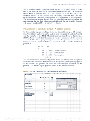
The Excel formulation is shown in Figure 3.5. When Excel Solver finds the optimal
solution to an LP problem, the Solver Results dialogue box (see Figure 3.6) appears
on the screen. This provides an option for different types of report on the
problem. The Answer report provides details of the optimal solution.

Figure 3.5 Excel Formulation for the M&D Chemicals Problem

Copyright 2014 Cengage Learning. All Rights Reserved. May not be copied, scanned, or duplicated, in whole or in part. Due to electronic rights, some third party content may be suppressed from the eBook and/or eChapter(s). Editorial review has
deemed that any suppressed content does not materially affect the overall learning experience. Cengage Learning reserves the right to remove additional content at any time if subsequent rights restrictions require it.