Page 126 -

106 CHAPTER 3 LINEAR PROGRAMMING: SENSITIVITY ANALYSIS AND INTERPRETATION OF SOLUTION

The Modified GulfGolf Problem
The original GulfGolf problem is restated as follows:

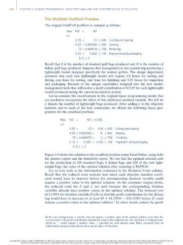
Max 10S þ 9D
s:t:
0:7S þ 1D 630 Cutting and dyeing
0:5S þ 0:83333D 600 Sewing
1S þ 0:66667D 708 Finishing
0:1S þ 0:25D 135 Inspection and packaging
S; D 0
Recall that S is the number of standard golf bags produced and D is the number of
deluxe golf bags produced. Suppose that management is also considering producing a
lightweight model designed specifically for women golfers. The design department
estimates that each new lightweight model will require 0.8 hours for cutting and
dyeing, one hour for sewing, one hour for finishing and 0.25 hours for inspection
and packaging. Because of the unique capabilities designed into the new model,
management feels they will realize a profit contribution of $12.85 for each lightweight
model produced during the current production period.
Let us consider the modifications in the original linear programming model that
are needed to incorporate the effect of this additional decision variable. We will let
L denote the number of lightweight bags produced. After adding L to the objective
function and to each of the four constraints, we obtain the following linear pro-
gramme for the modified problem:

Max 10S þ 9D þ 12:85L
s:t:
0:7S þ 1D þ 0:8L 630 Cutting and dyeing
0:5S þ 0:83333D þ 1L 600 Sewing
1S þ 0:66667D þ 1L 708 Finishing
0:1S þ 0:25D þ 0:25L 135 Inspection and packaging
S; D; L 0

Figure 3.9 shows the solution to the modified problem using Excel Solver, using both
the Answer report and the Sensitivity report. We see that the optimal solution calls
for the production of 280 standard bags, 0 deluxe bags and 428 of the new light-
weight bags; the value of the optimal solution after rounding is $8299.80.
Let us now look at the information contained in the Reduced Costs column.
Recall that the reduced costs indicate how much each objective function coeffi-
cient would have to improve before the corresponding decision variable could
assume a positive value in the optimal solution. As the computer output shows,
the reduced costs for S and L are zero because the corresponding decision
variables already have positive values in the optimal solution. The reduced cost
of 1.15003 for decision variable D tells us that the profit contribution for the deluxe
bag would have to increase to at least $9 + $1.15003 ¼ $10.15003 before Dcould
3
assume a positive value in the optimal solution. In other words, unless the profit

3
In the case of degeneracy, a variable may not assume a positive value in the optimal solution even when the
improvement in the profit contribution exceeds the value of the reduced cost. Our definition of reduced costs,
stated as ‘. . . could assume a positive value. . .,’ provides for such special cases. More advanced texts on
mathematical programming discuss these special types of situations.

Copyright 2014 Cengage Learning. All Rights Reserved. May not be copied, scanned, or duplicated, in whole or in part. Due to electronic rights, some third party content may be suppressed from the eBook and/or eChapter(s). Editorial review has
deemed that any suppressed content does not materially affect the overall learning experience. Cengage Learning reserves the right to remove additional content at any time if subsequent rights restrictions require it.