Page 123 -

SENSITIVITY ANALYSIS: COMPUTER SOLUTION 103

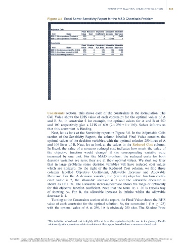
Figure 3.8 Excel Solver Sensitivity Report for the M&D Chemicals Problem

Constraints section. This shows each of the constraints in the formulation. The
Cell Valueshows theLHSvalueofeach constraintfor theoptimal values of A
and B. So, in constraint 2 for example, the optimal values for A and B of 250
and 100 respectively give a LHS of 600 (2 250 + 1 100). Solver informs us
that this constraint is Binding.
Next, let us look at the Sensitivity report in Figure 3.8. In the Adjustable Cells
section of the Sensitivity Report, the column labelled Final Value contains the
optimal values of the decision variables, with the optimal solution 250 litres of A
and 100 litres of B. Next, let us look at the values in the Reduced Cost column.
In Excel, the value of a nonzero reduced cost indicates how much the value of
the objective function would change 2 if the corresponding variable were
increased by one unit. For the M&D problem, the reduced costs for both
decision variables are zero; they are at their optimal values. We shall see later
that in large problems some decision variables will have reduced cost values
which are nonzero. To the right of the Reduced Cost column, we find three
columns labelled Objective Coefficient, Allowable Increase and Allowable
Decrease. For the A decision variable, the (current) objective function coeffi-
cient value is 2, the allowable increase is 1 and the allowable decrease is
shown as 1E + 30. The allowable increase/decrease shows the range of optimality
for this objective function coefficient. Note that the term 1E + 30 is Excel’s way
of showing 1. For B, the allowable increase in infinite whilst the allowable
decrease is 1.
Turning to the Constraints section of the report, the Final Value shows the RHS
value of each constraint for the optimal solution. So, for constraint 1 (1A 125)
with the optimal value of A at 250, 1A is obviously 250 also. The Shadow Price

2
This definition of reduced cost is slightly different from (but equivalent to) the one in the glossary. Excel’s
solution algorithm permits variables in solution at their upper bound to have a nonzero reduced cost.

Copyright 2014 Cengage Learning. All Rights Reserved. May not be copied, scanned, or duplicated, in whole or in part. Due to electronic rights, some third party content may be suppressed from the eBook and/or eChapter(s). Editorial review has
deemed that any suppressed content does not materially affect the overall learning experience. Cengage Learning reserves the right to remove additional content at any time if subsequent rights restrictions require it.