Page 171 -

PRODUCTION MANAGEMENT APPLICATIONS 151

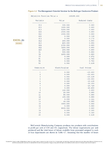
Figure 4.2 The Management Scientist Solution for the Bollinger Electronics Problem

Objective Function Value = 225295.000

Variable Value Reduced Costs
-------------- --------------- -----------------
X11 500.000 0.000
X12 3200.000 0.000
X13 5200.000 0.000
X21 2500.000 0.000
X22 2000.000 0.000
X23 0.000 0.128
S11 0.000 0.172
EXCEL file S12 200.000 0.000
S13 400.000 0.000
BOLLINGER
S21 1700.000 0.000
S22 3200.000 0.000
S23 200.000 0.000
I1 500.000 0.000
I2 2200.000 0.000
I3 0.000 0.072
D1 0.000 0.700
D2 0.000 0.700
D3 0.000 0.628

Constraint Slack/Surplus Dual Prices
-------------- --------------- -----------------
1 0.000 –20.000
2 0.000 –10.000
3 0.000 –20.128
4 0.000 –10.150
5 0.000 –20.428
6 0.000 –10.300
7 0.000 –20.728
8 0.000 –10.450
9 150.000 0.000
10 20.000 0.000
11 80.000 0.000
12 100.000 0.000
13 0.000 1.111
14 40.000 0.000
15 4900.000 0.000
16 0.000 0.000
17 8600.000 0.000
18 0.000 0.500
19 0.000 0.500
20 0.000 0.428

McCormick Manufacturing Company produces two products with contributions
to profit per unit of E10 and E9, respectively. The labour requirements per unit
produced and the total hours of labour available from personnel assigned to each
of four departments are shown in Table 4.7. Assuming that the number of hours

Copyright 2014 Cengage Learning. All Rights Reserved. May not be copied, scanned, or duplicated, in whole or in part. Due to electronic rights, some third party content may be suppressed from the eBook and/or eChapter(s). Editorial review has
deemed that any suppressed content does not materially affect the overall learning experience. Cengage Learning reserves the right to remove additional content at any time if subsequent rights restrictions require it.