Page 166 -

146 CHAPTER 4 LINEAR PROGRAMMING APPLICATIONS

another. Increasing production, for example, may need extra staff, extra supplies;
decreasing production may mean laying off staff temporarily and cancelling supplies
that have been ordered. Such short-term actions may cost the company money.
In the remainder of this section, we show how to formulate a linear programming
model of the production and inventory process for Bollinger Electronics to minimize
the total cost.
To develop the model, we let x im denote the production volume in units for
product i in month m. Here i ¼ 1, 2, and m ¼ 1, 2, 3; i ¼ 1 refers to component
322A, i ¼ 2 refers to component 802B, m ¼ 1 refers to April, m ¼ 2 refers to May
and m ¼ 3 refers to June. The purpose of the double subscript is to provide a more
descriptive notation. We could simply use x 6 to represent the number of units of
product 2 produced in month 3, but x 23 is more descriptive, identifying directly the
product and month represented by the variable.
Component 322A costs E20 per unit produced and component 802B costs E10
per unit produced, so the total production cost part of the objective function is:

Total production cost ¼ 20x 11 þ 20x 12 þ 20x 13 þ 10x 21 þ 10x 22 þ 10x 23
Because the production cost per unit is the same each month, we don’t need to
include the production costs in the objective function; that is, regardless of the
production schedule selected, the total production cost will remain the same. In
other words, production costs are not relevant costs for the production scheduling
decision under consideration. In cases in which the production cost per unit is
expected to change each month, the variable production costs per unit per month
must be included in the objective function. The solution for the Bollinger Elec-
tronics problem will be the same whether these costs are included, therefore we
include them so that the value of the linear programming objective function will
include all the costs associated with the problem.
To incorporate the relevant inventory holding costs into the model, we let s im
denote the inventory level for product i at the end of month m. Bollinger determined
that on a monthly basis inventory holding costs are 1.5 per cent of the cost of the
product; that is, (0.015)(E20) ¼ E0.30 per unit for component 322A and
(0.015)(E10) ¼ E0.15 per unit for component 802B. A common assumption made
in using the linear programming approach to production scheduling is that monthly
ending inventories are an acceptable approximation to the average inventory levels
throughout the month. Making this assumption, we write the inventory holding cost
portion of the objective function as:

Inventory holding cost ¼ 0:30s 11 þ 0:30s 12 þ 0:30s 13 þ 0:15s 21 þ 0:15s 22 þ 0:15s 23
To incorporate the costs of fluctuations in production levels from month to month,
we need to define two additional variables:

I m ¼ increase in the total production level necessary during month m
D m ¼ decrease in the total production level necessary during month m

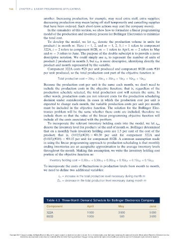
Table 4.3 Three-Month Demand Schedule for Bollinger Electronics Company
Component April May June

322A 1 000 3 000 5 000
802B 1 000 500 3 000

Copyright 2014 Cengage Learning. All Rights Reserved. May not be copied, scanned, or duplicated, in whole or in part. Due to electronic rights, some third party content may be suppressed from the eBook and/or eChapter(s). Editorial review has
deemed that any suppressed content does not materially affect the overall learning experience. Cengage Learning reserves the right to remove additional content at any time if subsequent rights restrictions require it.