Page 192 -

172 CHAPTER 4 LINEAR PROGRAMMING APPLICATIONS

Max 0:073A þ 0:103P þ 0:064M þ 0:075H þ 0:045G
s:t:
A þ P þ M þ H þ G ¼ 100 000 Available funds
A þ P 50 000 Oil industry maximum
M þ H 50 000 Steel industry maximum
0:25M 0:25H þ G 0 Government
bonds minimum
0:6A þ 0:4P 0 Pacific Oil restriction
A; P; M; H; G 0
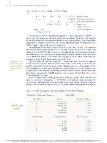
The optimal solution to this linear programme is shown in Figure 4.8. Table 4.15
shows how the funds are divided among the securities. Note that the optimal
solution indicates that the portfolio should be diversified among all the investment
opportunities except Midwest Steel. The projected annual return for this portfolio is
E8000, which is an overall return of 8 per cent.
The optimal solution shows the dual price for constraint 3 is zero. The reason is
that the steel industry maximum isn’t a binding constraint; increases in the steel
industry limit of E50 000 will not improve the value of the optimal solution. Indeed,
the slack variable for this constraint shows that the current steel industry investment
is E10 000 below its limit of E50 000. The dual prices for the other constraints are
nonzero, indicating that these constraints are binding.
The dual price for the The dual price of 0.069 for constraint 1 shows that the value of the optimal
available funds constraint solution can be increased by 0.069 if one more euro can be made available for the
provides information on
the rate of return from portfolio investment. If more funds can be obtained at a cost of less than 6.9 per
additional investment cent, management should consider obtaining them. However, if a return in excess of
funds. 6.9 per cent can be obtained by investing funds elsewhere (other than in these five
securities), management should question the wisdom of investing the entire
E100 000 in this portfolio.
Similar interpretations can be given to the other dual prices. Note that the dual
price for constraint 4 is negative at 0.024. This result indicates that increasing the
value on the right-hand side of the constraint by one unit can be expected to worsen
the value of the optimal solution by 0.024. In terms of the optimal portfolio, then, if

Figure 4.8 The Management Scientist Solution for the Welte Problem

Objective Function Value = 8000.000
Variable Value Reduced Costs
-------------- --------------- -----------------
A 20000.000 0.000
EXCEL file P 30000.000 0.000
M 0.000 0.011
WELTE
H 40000.000 0.000
G 10000.000 0.000

Constraint Slack/Surplus Dual Prices
-------------- --------------- -----------------
1 0.000 0.069
2 0.000 0.022
3 10000.000 0.000
4 0.000 –0.024
5 0.000 0.030

Copyright 2014 Cengage Learning. All Rights Reserved. May not be copied, scanned, or duplicated, in whole or in part. Due to electronic rights, some third party content may be suppressed from the eBook and/or eChapter(s). Editorial review has
deemed that any suppressed content does not materially affect the overall learning experience. Cengage Learning reserves the right to remove additional content at any time if subsequent rights restrictions require it.