Page 254 -

234 CHAPTER 5 LINEAR PROGRAMMING: THE SIMPLEX METHOD

x 1 x 2 s 1 s 2 s 3 s 4
Basis c B 50 40 0 0 0 0
0 0 3.125 1 0 0.375 0 37.5
s 1
0 0 1 0 1 0 0 20
s 2
0 0 0.375 0 0 0.125 1 12.5
s 4
x 1 50 1 0.625 0 0 0.125 0 37.5
z j 50 31.25 0 0 6.250 0 1 875
0 8.75 0 0 6.250 0
c j – z j

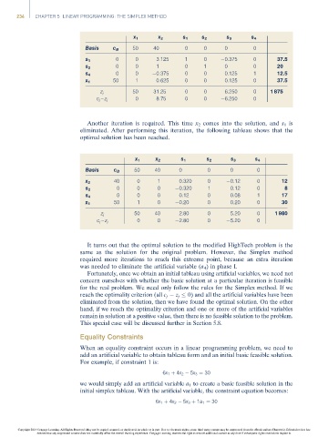
Another iteration is required. This time x 2 comes into the solution, and s 1 is
eliminated. After performing this iteration, the following tableau shows that the
optimal solution has been reached.

x 1 x 2 s 1 s 2 s 3 s 4
Basis c B 50 40 0 0 0 0
40 0 1 0.320 0 0.12 0 12
x 2
0 0 0 0.320 1 0.12 0 8
s 2
0 0 0 0.12 0 0.08 1 17
s 4
50 1 0 0.20 0 0.20 0 30
x 1
50 40 2.80 0 5.20 0 1 980
z j
0 0 2.80 0 5.20 0
c j – z j
It turns out that the optimal solution to the modified HighTech problem is the
same as the solution for the original problem. However, the Simplex method
required more iterations to reach this extreme point, because an extra iteration
was needed to eliminate the artificial variable (a 4 ) in phase I.
Fortunately, once we obtain an initial tableau using artificial variables, we need not
concern ourselves with whether the basic solution at a particular iteration is feasible
for the real problem. We need only follow the rules for the Simplex method. If we
reach the optimality criterion (all c j z j 0) and all the artificial variables have been
eliminated from the solution, then we have found the optimal solution. On the other
hand, if we reach the optimality criterion and one or more of the artificial variables
remain in solution at a positive value, then there is no feasible solution to the problem.
This special case will be discussed further in Section 5.8.

Equality Constraints
When an equality constraint occurs in a linear programming problem, we need to
add an artificial variable to obtain tableau form and an initial basic feasible solution.
For example, if constraint 1 is:

6x 1 þ 4x 2 5x 3 ¼ 30
we would simply add an artificial variable a 1 to create a basic feasible solution in the
initial simplex tableau. With the artificial variable, the constraint equation becomes:

6x 1 þ 4x 2 5x 3 þ 1a 1 ¼ 30

Copyright 2014 Cengage Learning. All Rights Reserved. May not be copied, scanned, or duplicated, in whole or in part. Due to electronic rights, some third party content may be suppressed from the eBook and/or eChapter(s). Editorial review has
deemed that any suppressed content does not materially affect the overall learning experience. Cengage Learning reserves the right to remove additional content at any time if subsequent rights restrictions require it.