Page 259 -

SPECIAL CASES 239

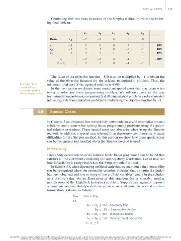
Continuing with two more iterations of the Simplex method provides the follow-
ing final tableau:

x 1 x 2 s 1 s 2 s 3
Basis c B 2 3 0 0 0

x 1 2 1 0 0 1 1 250
x 2 3 0 1 0 2 1 100
s 1 0 0 0 1 1 1 125
2 3 0 4 1 800
z j
0 0 0 4 1
c j – z j

The value of the objective function 800 must be multiplied by 1 to obtain the
value of the objective function for the original minimization problem. Thus, the
Try Problem 14 for minimum total cost of the optimal solution is E800.
practise solving a In the next section we discuss some important special cases that may occur when
minimization problem
with the Simplex method. trying to solve any linear programming problem. We will only consider the case
for maximization problems, recognizing that all minimization problems can be converted
into an equivalent maximization problem by multiplying the objective function by 1.

5.8 Special Cases

In Chapter 2 we discussed how infeasibility, unboundedness and alternative optimal
solutions could occur when solving linear programming problems using the graph-
ical solution procedure. These special cases can also arise when using the Simplex
method. In addition, a special case referred to as degeneracy can theoretically cause
difficulties for the Simplex method. In this section we show how these special cases
can be recognized and handled when the Simplex method is used.

Infeasibility
Infeasibility occurs whenever no solution to the linear programme can be found that
satisfies all the constraints, including the nonnegativity constraints. Let us now see
how infeasibility is recognized when the Simplex method is used.
In Section 5.6, when discussing artificial variables, we mentioned that infeasibility
can be recognized when the optimality criterion indicates that an optimal solution
has been obtained and one or more of the artificial variables remain in the solution
at a positive value. As an illustration of this situation, let us consider another
modification of the HighTech Industries problem. Suppose management imposed
a minimum combined total production requirement of 50 units. The revised problem
formulation is shown as follows.
Max 50x 1 þ 40x 2
s:t:
3x 1 þ 5x 2 150 Assembly time
1x 2 20 Ultraportable display
8x 1 þ 5x 2 300 Warehouse space
1x 1 þ 1x 2 50 Minimum total production
x 1 ; x 2 0

Copyright 2014 Cengage Learning. All Rights Reserved. May not be copied, scanned, or duplicated, in whole or in part. Due to electronic rights, some third party content may be suppressed from the eBook and/or eChapter(s). Editorial review has
deemed that any suppressed content does not materially affect the overall learning experience. Cengage Learning reserves the right to remove additional content at any time if subsequent rights restrictions require it.