Page 264 -

244 CHAPTER 5 LINEAR PROGRAMMING: THE SIMPLEX METHOD

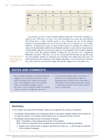
x 1 x 2 s 1 s 2 s 3
Basis c B 50 40 0 0 0
40 0 1 0.32 0 0.12 20
x 2
0 0 0 0.32 1 0.12 0
s 2
50 1 0 0.20 0 0.20 25
x 1
z j 50 40 2.80 0 5.20 2 050
c j – z j 0 0 2.80 0 5.20

As expected, we have a basic feasible solution with one of the basic variables, s 2 ,
equal to zero. Whenever we have a tie in the minimum b i /a ij ratio, the next tableau
will always have a basic variable equal to zero. Because we are at the optimal
solution in the preceding case, we do not care that s 2 is in solution at a zero value.
However, if degeneracy occurs at some iteration prior to reaching the optimal sol-
ution, it is theoretically possible for the Simplex method to cycle; that is, the procedure
could possibly alternate between the same set of nonoptimal basic feasible solutions
and never reach the optimal solution. Cycling has not proven to be a significant
difficulty in practice. Therefore, we do not recommend introducing any special steps
The Simplex method was into the Simplex method to eliminate the possibility that degeneracy will occur. If
chosen as one of the
twentieth-century’s top while performing the iterations of the simplex algorithm a tie occurs for the minimum
20 algorithms b i /a ij ratio, then we recommend simply selecting the upper row as the pivot row.

NOTES AND COMMENTS

1 We stated that infeasibility is recognized when the 2 An unbounded feasible region must exist for a
stopping rule is encountered but one or more problem to be unbounded, but it does not
artificial variables are in solution at a positive guarantee that a problem will be unbounded. A
value. This requirement does not necessarily minimization problem may be bounded whereas
mean that all artificial variables must be a maximization problem with the same feasible
non-basic to have a feasible solution. An artificial region is unbounded.
variable could be in solution at a zero value.

Summary
In this chapter we introduced the Simplex method as an algorithm for solving LP problems.

l The Simplex method follows a set of standard steps to find a basic, feasible solution and to search for
an improved solution. The Simplex method stops when no improved solution is found.
l The Simplex method steps can be summarized as follows:
Step 1: Formulate a linear programming model of the problem.
Step 2: Define an equivalent linear programme by performing the following operations:
a. Multiply each constraint with a negative right-hand side value by 1, and change the direction
of the constraint inequality.

Copyright 2014 Cengage Learning. All Rights Reserved. May not be copied, scanned, or duplicated, in whole or in part. Due to electronic rights, some third party content may be suppressed from the eBook and/or eChapter(s). Editorial review has
deemed that any suppressed content does not materially affect the overall learning experience. Cengage Learning reserves the right to remove additional content at any time if subsequent rights restrictions require it.