Page 287 -

DUALITY 267

4 The right-hand sides of the primal constraints become the objective function
coefficients in the dual.
5 The objective function coefficients of the primal become the right-hand sides
of the dual constraints.
6 The constraint coefficients of the ith primal variable become the coefficients in
the ith constraint of the dual.
Try part (a) of Problem These six statements are the general requirements that must be satisfied when
12 for practise in finding converting a maximization problem in canonical form to its associated dual: a
the dual of a
maximization problem in minimization problem in canonical form. Even though these requirements may seem
canonical form. cumbersome at first, practise with a few simple problems will show that the primal–
dual conversion process is relatively easy to implement.
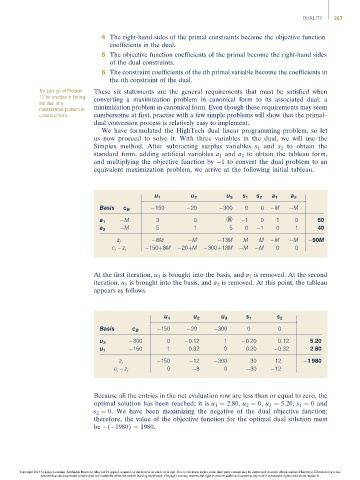
We have formulated the HighTech dual linear programming problem, so let
us now proceed to solve it. With three variables in the dual, we will use the
Simplex method. After subtracting surplus variables s 1 and s 2 to obtain the
standard form, adding artificial variables a 1 and a 2 to obtain the tableau form,
and multiplying the objective function by 1 to convert the dual problem to an
equivalent maximization problem, we arrive at the following initial tableau.

u 1 u 2 u 3 s 1 s 2 a 1 a 2
Basis c B 150 20 300 0 0 M M
M 3 0 ‡ 1 0 1 0 50
a 1
M 5 1 5 0 1 0 1 40
a 2
z j 8M M 13M M M M M 90M
c j – z j 150þ8M 20þM 300þ13M M M 0 0

At the first iteration, u 3 is brought into the basis, and a 1 is removed. At the second
iteration, u 1 is brought into the basis, and a 2 is removed. At this point, the tableau
appears as follows.

u 1 u 2 u 3 s 1 s 2
Basis c B 150 20 300 0 0

u 3 300 0 0.12 1 0.20 0.12 5.20
150 1 0.32 0 0.20 0.32 2.80
u 1
150 12 300 30 12 1 980
z j
0 8 0 30 12
c j – z j

Because all the entries in the net evaluation row are less than or equal to zero, the
optimal solution has been reached; it is u 1 ¼ 2.80, u 2 ¼ 0, u 3 ¼ 5.20, s 1 ¼ 0and
s 2 ¼ 0. We have been maximizing the negative of the dual objective function;
therefore, the value of the objective function for the optimal dual solution must
be ( 1980) ¼ 1980.

Copyright 2014 Cengage Learning. All Rights Reserved. May not be copied, scanned, or duplicated, in whole or in part. Due to electronic rights, some third party content may be suppressed from the eBook and/or eChapter(s). Editorial review has
deemed that any suppressed content does not materially affect the overall learning experience. Cengage Learning reserves the right to remove additional content at any time if subsequent rights restrictions require it.