Page 282 -

262 CHAPTER 6 SIMPLEX-BASED SENSITIVITY ANALYSIS AND DUALITY

dual price, the value of the optimal solution has increased by 10(E2.80) ¼ E28, from
E1980 to E2008.
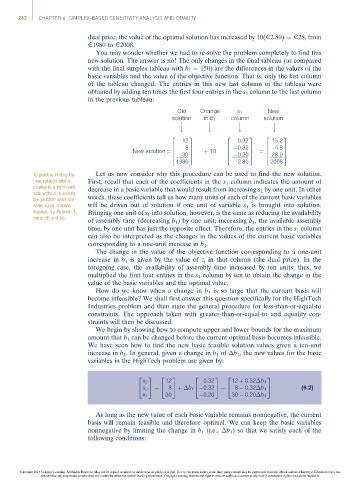
You may wonder whether we had to re-solve the problem completely to find this
new solution. The answer is no! The only changes in the final tableau (as compared
with the final simplex tableau with b 1 ¼ 150) are the differences in the values of the
basic variables and the value of the objective function. That is, only the last column
of the tableau changed. The entries in this new last column of the tableau were
obtained by adding ten times the first four entries in the s 1 column to the last column
in the previous tableau:
Old Change s 1 New
solution in b 1 column solution
# # # #
2 3 2 3 2 3
12 0:32 15:2
6 8 7 6 0:32 7 6 4:8 7
New solution ¼ 6 30 7 þ 10 6 0:20 7 ¼ 6 28:0 7
5
4
5
4
5
4
1980 2:80 2008
To practise finding the Let us now consider why this procedure can be used to find the new solution.
new solution after a First, recall that each of the coefficients in the s 1 column indicates the amount of
change in a right-hand decrease in a basic variable that would result from increasing s 1 by one unit. In other
side without re-solving
the problem when the words, these coefficients tell us how many units of each of the current basic variables
same basis remains will be driven out of solution if one unit of variable s 1 is brought into solution.
feasible, try Problem 3, Bringing one unit of s 1 into solution, however, is the same as reducing the availability
parts (d) and (e).
of assembly time (decreasing b 1 ) by one unit; increasing b 1 , the available assembly
time, by one unit has just the opposite effect. Therefore, the entries in the s 1 column
can also be interpreted as the changes in the values of the current basic variables
corresponding to a one-unit increase in b 1 .
The change in the value of the objective function corresponding to a one-unit
increase in b 1 is given by the value of z j in that column (the dual price). In the
foregoing case, the availability of assembly time increased by ten units; thus, we
multiplied the first four entries in the s 1 column by ten to obtain the change in the
value of the basic variables and the optimal value.
How do we know when a change in b 1 is so large that the current basis will
become infeasible? We shall first answer this question specifically for the HighTech
Industries problem and then state the general procedure for less-than-or-equal-to
constraints. The approach taken with greater-than-or-equal-to and equality con-
straints will then be discussed.
We begin by showing how to compute upper and lower bounds for the maximum
amount that b 1 can be changed before the current optimal basis becomes infeasible.
We have seen how to find the new basic feasible solution values given a ten-unit
increase in b 1 . In general, given a change in b 1 of b 1 , the new values for the basic
variables in the HighTech problem are given by:

2 3 2 3 2 3 2 3
x 2 12 0:32 12 þ 0:32 b 1
4
4 5 ¼ 4 8 5 þ b 1 0:32 5 ¼ 4 5 (6:2)
s 2 8 0:32 b 1
x 1 30 0:20 30 0:20 b 1
As long as the new value of each basic variable remains nonnegative, the current
basis will remain feasible and therefore optimal. We can keep the basic variables
nonnegative by limiting the change in b 1 (i.e., b 1 ) so that we satisfy each of the
following conditions:

Copyright 2014 Cengage Learning. All Rights Reserved. May not be copied, scanned, or duplicated, in whole or in part. Due to electronic rights, some third party content may be suppressed from the eBook and/or eChapter(s). Editorial review has
deemed that any suppressed content does not materially affect the overall learning experience. Cengage Learning reserves the right to remove additional content at any time if subsequent rights restrictions require it.