Page 278 -

258 CHAPTER 6 SIMPLEX-BASED SENSITIVITY ANALYSIS AND DUALITY

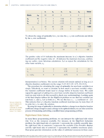
x 1 x 2 s 1 s 2 s 3 Value
Basis c B 50 40 0 0 0
40 0 1 0.32 0 0.12 12
x 2
0 0 0 0.32 1 0.12 8
s 2
50 1 0 0.20 0 0.20 30
x 1
z j 50 40 2.8 0 5.2 1 980
c j –z j 0 0 2.8 0 5.2

To obtain the range of optimality for x 1 we take the c j – z j row coefficients and divide
by the x 1 row coefficients.

0 0 2.8 0 5.2
c j – z j
1 0 0.20 0 0.20
x 1
c j – cz j /x 1 0 0 14 0 26

The positive value of 14 indicates the maximum increase in x 1 ’s objective function
coefficient and the negative value of 26 indicates the maximum decrease, confirm-
ing our earlier, more laborious calculations. Let us repeat the calculations for the
other basic variable, x 2 .

0 0 2.8 0 5.2
c j – z j
0 1 0.32 0 0.12
x 2
0 0 8.75 0 43.3
c j – cz j /x 2

Interpretation is as before. The current solution will remain optimal as long as x 2 ’s
objective function coefficient is in the range 31.25–83.3 (40 8.75, 40+43.3).
The procedure for calculating the range of optimality for non-basic variables is as
simple. Effectively, we want to calculate by how much a non-basic variable’s objec-
tive function coefficient would need to change before it became basic. We could
repeat the approach of adding k to a non-basic variable objective function coefficient
(and you may wish to do this yourself to check your understanding). Looking again
at the final simplex tableau for the HighTech problem we see that two variables are
non-basic: s 1 and s 2 . Let us look at s 1 . We see this has a c j – z j coefficient of 2.8.
Can you compute the This indicates that s 1 ’s objective function coefficient must increase by more than 2.8
range of optimality for in order for s 1 to enter the solution.
objective function By using the range of optimality to determine whether a change in an objective function
coefficients by working
with the final simplex coefficient is large enough to cause a change in the optimal solution, we can often avoid the
tableau? Try Problem 1. process of formulating and solving a modified linear programming problem.

Right-Hand Side Values
In many linear programming problems, we can interpret the right-hand side values
(the ‘b i ’s) as the resources available. For instance, in the HighTech Industries
problem, the right-hand side of constraint 1 represents the available assembly time,
the right-hand side of constraint 2 represents the available Ultra Portable displays
and the right-hand side of constraint 3 represents the available warehouse space.
Dual prices provide information on the value of additional resources in these cases;

Copyright 2014 Cengage Learning. All Rights Reserved. May not be copied, scanned, or duplicated, in whole or in part. Due to electronic rights, some third party content may be suppressed from the eBook and/or eChapter(s). Editorial review has
deemed that any suppressed content does not materially affect the overall learning experience. Cengage Learning reserves the right to remove additional content at any time if subsequent rights restrictions require it.