Page 275 -

SENSITIVITY ANALYSIS WITH THE SIMPLEX TABLEAU 255

In Chapter 3 we saw how simple sensitivity analysis could be applied to the optimal
solution of an LP problem to examine how marginal changes in the problem might
affect the current solution. In practice it is the sensitivity analysis information that
may be of most value to management decision makers. In this chapter we look at
sensitivity analysis in detail and show how the Simplex solution can be used to
produce this information.

6.1 Sensitivity Analysis with the Simplex Tableau

The usual sensitivity analysis for linear programmes involves calculating ranges for the
objective function coefficients and the right-hand side values, as well as the dual prices.

Objective Function Coefficients
Sensitivity analysis for an objective function coefficient involves placing a range on
the coefficient’s value. We call this range the range of optimality. As long as the
actual value of the objective function coefficient is within the range of optimality, the
current basic feasible solution will remain optimal. The range of optimality for a basic
variable defines the objective function coefficient values for which that variable will
remain part of the current optimal basic feasible solution. The range of optimality
for a nonbasic variable defines the objective function coefficient values for which
that variable will remain nonbasic.
In calculating the range of optimality for an objective function coefficient, all
other coefficients in the problem are assumed to remain at their original values; in
other words, only one coefficient is allowed to change at a time. To illustrate the
process of computing ranges for objective function coefficients, recall the HighTech
Industries problem introduced in Chapter 5. The linear programme for this problem
is restated as follows:
Max 50x 1 þ 40x 2
s:t:
3x 1 þ 5x 2 150 Assembly time
1x 2 20 UltraPortable display
8x 1 þ 5x 2 300 Warehouse capacity
x 1 ; x 2 0
where
x 1 ¼ number of units of the Deskpro
x 2 ¼ number of units of the UltraPortable

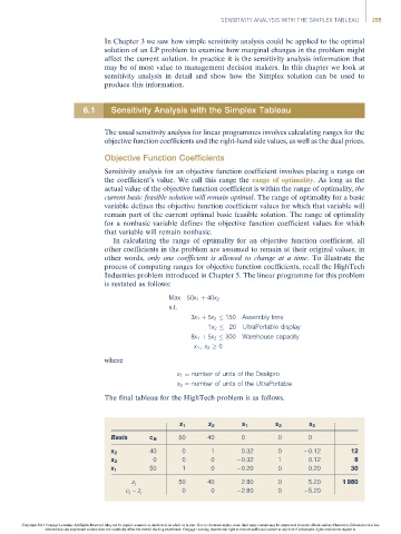
The final tableau for the HighTech problem is as follows.

x 1 x 2 s 1 s 2 s 3
Basis c B 50 40 0 0 0

x 2 40 0 1 0.32 0 0.12 12
0 0 0 0.32 1 0.12 8
s 2
50 1 0 0.20 0 0.20 30
x 1
50 40 2.80 0 5.20 1 980
z j
0 0 2.80 0 5.20
c j – z j

Copyright 2014 Cengage Learning. All Rights Reserved. May not be copied, scanned, or duplicated, in whole or in part. Due to electronic rights, some third party content may be suppressed from the eBook and/or eChapter(s). Editorial review has
deemed that any suppressed content does not materially affect the overall learning experience. Cengage Learning reserves the right to remove additional content at any time if subsequent rights restrictions require it.