Page 277 -

SENSITIVITY ANALYSIS WITH THE SIMPLEX TABLEAU 257

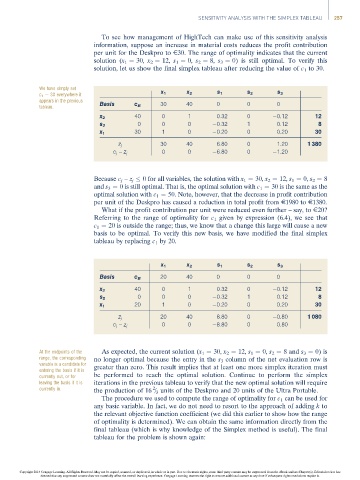
To see how management of HighTech can make use of this sensitivity analysis
information, suppose an increase in material costs reduces the profit contribution
per unit for the Deskpro to E30. The range of optimality indicates that the current
solution (x 1 ¼ 30, x 2 ¼ 12, s 1 ¼ 0, s 2 ¼ 8, s 3 ¼ 0) is still optimal. To verify this
solution, let us show the final simplex tableau after reducing the value of c 1 to 30.

We have simply set
c 1 ¼ 30 everywhere it x 1 x 2 s 1 s 2 s 3
appears in the previous
tableau. Basis c B 30 40 0 0 0
x 2 40 0 1 0.32 0 0.12 12
s 2 0 0 0 0.32 1 0.12 8
30 1 0 0.20 0 0.20 30
x 1
30 40 6.80 0 1.20 1 380
z j
0 0 6.80 0 1.20
c j – z j

Because c j – z j 0 for all variables, the solution with x 1 ¼ 30, x 2 ¼ 12, s 1 ¼ 0, s 2 ¼ 8
and s 3 ¼ 0 is still optimal. That is, the optimal solution with c 1 ¼ 30 is the same as the
optimal solution with c 1 ¼ 50. Note, however, that the decrease in profit contribution
per unit of the Deskpro has caused a reduction in total profit from E1980 to E1380.
What if the profit contribution per unit were reduced even further – say, to E20?
Referring to the range of optimality for c 1 given by expression (6.4), we see that
c 1 ¼ 20 is outside the range; thus, we know that a change this large will cause a new
basis to be optimal. To verify this new basis, we have modified the final simplex
tableau by replacing c 1 by 20.

x 1 x 2 s 1 s 2 s 3
Basis c B 20 40 0 0 0

x 2 40 0 1 0.32 0 0.12 12
s 2 0 0 0 0.32 1 0.12 8
x 1 20 1 0 0.20 0 0.20 30
20 40 8.80 0 0.80 1 080
z j
0 0 8.80 0 0.80
c j – z j

At the endpoints of the As expected, the current solution (x 1 ¼ 30, x 2 ¼ 12, s 1 ¼ 0, s 2 ¼ 8 and s 3 ¼ 0) is
range, the corresponding no longer optimal because the entry in the s 3 column of the net evaluation row is
variable is a candidate for greater than zero. This result implies that at least one more simplex iteration must
entering the basis if it is
currently out, or for be performed to reach the optimal solution. Continue to perform the simplex
leaving the basis if it is iterations in the previous tableau to verify that the new optimal solution will require
currently in. the production of 16 / 3 units of the Deskpro and 20 units of the Ultra Portable.
2
The procedure we used to compute the range of optimality for c 1 can be used for
any basic variable. In fact, we do not need to resort to the approach of adding k to
the relevant objective function coefficient (we did this earlier to show how the range
of optimality is determined). We can obtain the same information directly from the
final tableau (which is why knowledge of the Simplex method is useful). The final
tableau for the problem is shown again:

Copyright 2014 Cengage Learning. All Rights Reserved. May not be copied, scanned, or duplicated, in whole or in part. Due to electronic rights, some third party content may be suppressed from the eBook and/or eChapter(s). Editorial review has
deemed that any suppressed content does not materially affect the overall learning experience. Cengage Learning reserves the right to remove additional content at any time if subsequent rights restrictions require it.