Page 281 -

SENSITIVITY ANALYSIS WITH THE SIMPLEX TABLEAU 261

Table 6.1 Tableau Location of Dual Price by Constraint Type
Constraint Type Dual Price Given by
z j value for the slack variable associated with the constraint
Negative of the z j value for the surplus variable associated with the
constraint
¼ z j value for the artificial variable associated with the constraint

Table 6.2 Dual Prices For M&D Chemicals Problem

Constraint Constraint Type Dual Price
Demand for product A 0
Total production 4
Processing time 1

constraint 2 shows that the marginal cost of increasing the total production require-
ment is E4 per unit. Finally, the dual price of one for the third constraint shows that
the per-unit value of additional processing time is E1.

Range of Feasibility As we have just seen, the z j row in the final tableau can be used
to determine the dual price and, as a result, predict the change in the value of the
objective function corresponding to a unit change in a b i . This interpretation is only
valid, however, as long as the change in b i is not large enough to make the current
basic solution infeasible. Thus, we will be interested in calculating a range of values
over which a particular b i can vary without any of the current basic variables
becoming infeasible (i.e., less than zero). This range of values will be referred to as
A change in b i does not the range of feasibility.
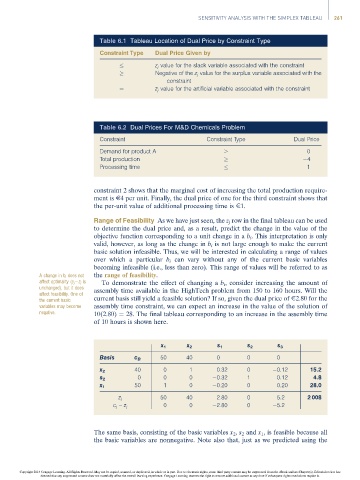
affect optimality (c j –z j is To demonstrate the effect of changing a b i , consider increasing the amount of
unchanged), but it does assembly time available in the HighTech problem from 150 to 160 hours. Will the
affect feasibility. One of
the current basic current basis still yield a feasible solution? If so, given the dual price of E2.80 for the
variables may become assembly time constraint, we can expect an increase in the value of the solution of
negative. 10(2.80) ¼ 28. The final tableau corresponding to an increase in the assembly time
of 10 hours is shown here.

x 1 x 2 s 1 s 2 s 3
Basis c B 50 40 0 0 0
x 2 40 0 1 0.32 0 0.12 15.2
s 2 0 0 0 0.32 1 0.12 4.8
x 1 50 1 0 0.20 0 0.20 28.0
50 40 2.80 0 5.2 2 008
z j
0 0 2.80 0 5.2
c j – z j

The same basis, consisting of the basic variables x 2 , s 2 and x 1 , is feasible because all
the basic variables are nonnegative. Note also that, just as we predicted using the

Copyright 2014 Cengage Learning. All Rights Reserved. May not be copied, scanned, or duplicated, in whole or in part. Due to electronic rights, some third party content may be suppressed from the eBook and/or eChapter(s). Editorial review has
deemed that any suppressed content does not materially affect the overall learning experience. Cengage Learning reserves the right to remove additional content at any time if subsequent rights restrictions require it.