Page 276 -

256 CHAPTER 6 SIMPLEX-BASED SENSITIVITY ANALYSIS AND DUALITY

Recall that when the Simplex method is used to solve a linear programme, an
optimal solution is recognized when all entries in the net evaluation row (c j – z j )
are 0. Because the preceding simplex tableau satisfies this criterion, the solution
shown is optimal. However, if a change in one of the objective function coefficients
were to cause one or more of the c j – z j values to become positive, then the current
solution would no longer be optimal; in such a case, one or more additional simplex
iterations would be necessary to find the new optimal solution. The range of optimality
for an objective function coefficient is determined by those coefficient values that main-
tain for all values of j.

c j z j 0 (6:1)

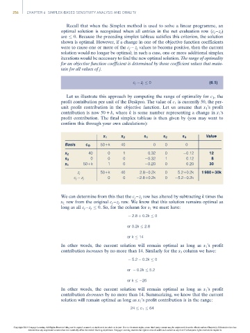
Let us illustrate this approach by computing the range of optimality for c 1 , the
profit contribution per unit of the Deskpro. The value of c 1 is currently 50, the per-
unit profit contribution in the objective function. Let us assume that x 1 ’s profit
contribution is now 50 + k, where k is some number representing a change in x 1 ’s
profit contribution. The final simplex tableau is then given by (you may want to
confirm this through your own calculations):

x 1 x 2 s 1 s 2 s 3 Value
Basis c B 50+k 40 0 0 0

x 2 40 0 1 0.32 0 0.12 12
s 2 0 0 0 0.32 1 0.12 8
x 1 50+k 1 0 0.20 0 0.20 30
50+k 40 2.8 0.2k 0 5.2+0.2k 1 980+30k
z j
0 0 2.8+0.2k 0 5.2 0.2k
c j – z j

We can determine from this that the c j – z j row has altered by subtracting k times the
x 1 row from the original c j – z j row. We know that this solution remains optimal as
long as all c j – z j 0. So, for the column for s 1 we must have:

2:8 þ 0:2k 0

or 0:2k 2:8
or k 14

In other words, the current solution will remain optimal as long as x 1 ’s profit
contribution increases by no more than 14. Similarly for the s 3 column we have:

5:2 0:2k 0

or 0:2k 5:2
or k 26

In other words, the current solution will remain optimal as long as x 1 ’s profit
contribution decreases by no more than 14. Summarizing, we know that the current
solution will remain optimal as long as x 1 ’s profit contribution is in the range:
24 c 1 64

Copyright 2014 Cengage Learning. All Rights Reserved. May not be copied, scanned, or duplicated, in whole or in part. Due to electronic rights, some third party content may be suppressed from the eBook and/or eChapter(s). Editorial review has
deemed that any suppressed content does not materially affect the overall learning experience. Cengage Learning reserves the right to remove additional content at any time if subsequent rights restrictions require it.