Page 279 -

SENSITIVITY ANALYSIS WITH THE SIMPLEX TABLEAU 259

the ranges over which these dual prices are valid are given by the ranges for the
right-hand side values.
Dual Prices In Chapter 3 we stated that the improvement in the value of the optimal
solution per unit increase in a constraint’s right-hand side value is called a dual price. 1
When the Simplex method is used to solve a linear programming problem, the values of
the dual prices are easy to obtain. They are found in the z j row of the final simplex tableau.
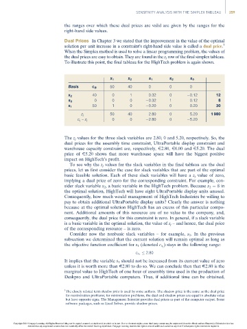
To illustrate this point, the final tableau for the HighTech problem is again shown.

x 1 x 2 s 1 s 2 s 3
Basis c B 50 40 0 0 0

40 0 1 0.32 0 0.12 12
x 2
0 0 0 0.32 1 0.12 8
s 2
x 1 50 1 0 0.20 0 0.20 30
z j 50 40 2.80 0 5.20 1 980
0 0 2.80 0 5.20
c j – z j

The z j values for the three slack variables are 2.80, 0 and 5.20, respectively. So, the
dual prices for the assembly time constraint, UltraPortable display constraint and
warehouse capacity constraint are, respectively, E2.80, E0.00 and E5.20. The dual
price of E5.20 shows that more warehouse space will have the biggest positive
impact on HighTech’s profit.
To see why the z j values for the slack variables in the final tableau are the dual
prices, let us first consider the case for slack variables that are part of the optimal
basic feasible solution. Each of these slack variables will have a z j value of zero,
implying a dual price of zero for the corresponding constraint. For example, con-
sider slack variable s 2 , a basic variable in the HighTech problem. Because s 2 ¼ 8in
the optimal solution, HighTech will have eight UltraPortable display units unused.
Consequently, how much would management of HighTech Industries be willing to
pay to obtain additional UltraPortable display units? Clearly the answer is nothing
because at the optimal solution HighTech has an excess of this particular compo-
nent. Additional amounts of this resource are of no value to the company, and,
consequently, the dual price for this constraint is zero. In general, if a slack variable
is a basic variable in the optimal solution, the value of z j – and hence, the dual price
of the corresponding resource – is zero.
Consider now the nonbasic slack variables – for example, s 1 . In the previous
subsection we determined that the current solution will remain optimal as long as
) stays in the following range:
the objective function coefficient for s 1 (denoted c s 1
2:80
c s 1
It implies that the variable s 1 should not be increased from its current value of zero
unless it is worth more than E2.80 to do so. We can conclude then that E2.80 is the
marginal value to HighTech of one hour of assembly time used in the production of
Deskpro and UltraPortable computers. Thus, if additional time can be obtained,

1
The closely related term shadow price is used by some authors. The shadow price is the same as the dual price
for maximization problems; for minimization problems, the dual and shadow prices are equal in absolute value
but have opposite signs. The Management Scientist provides dual prices as part of the computer output. Some
software packages, such as Excel Solver, provide shadow prices.

Copyright 2014 Cengage Learning. All Rights Reserved. May not be copied, scanned, or duplicated, in whole or in part. Due to electronic rights, some third party content may be suppressed from the eBook and/or eChapter(s). Editorial review has
deemed that any suppressed content does not materially affect the overall learning experience. Cengage Learning reserves the right to remove additional content at any time if subsequent rights restrictions require it.