Page 303 -

TRANSPORTATION PROBLEM: A NETWORK MODEL AND A LINEAR PROGRAMMING FORMULATION 283

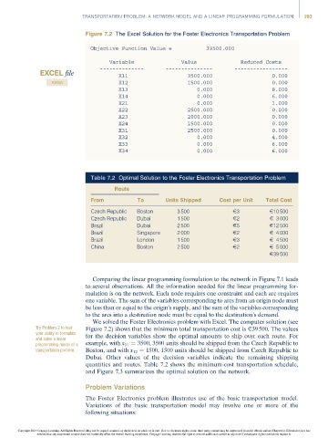
Figure 7.2 The Excel Solution for the Foster Electronics Transportation Problem

Objective Function Value = 39500.000

Variable Value Reduced Costs
-------------- --------------- -----------------
EXCEL file X11 3500.000 0.000
FOSTER X12 1500.000 0.000
X13 0.000 8.000
X14 0.000 6.000
X21 0.000 1.000
X22 2500.000 0.000
X23 2000.000 0.000
X24 1500.000 0.000
X31 2500.000 0.000
X32 0.000 4.000
X33 0.000 6.000
X34 0.000 6.000

Table 7.2 Optimal Solution to the Foster Electronics Transportation Problem

Route
From To Units Shipped Cost per Unit Total Cost
Czech Republic Boston 3 500 E3 E10 500
Czech Republic Dubai 1 500 E2 E 3 000
Brazil Dubai 2 500 E5 E12 500
Brazil Singapore 2 000 E2 E 4 000
Brazil London 1 500 E3 E 4 500
China Boston 2 500 E2 E 5 000
E39 500

Comparing the linear programming formulation to the network in Figure 7.1 leads
to several observations. All the information needed for the linear programming for-
mulation is on the network. Each node requires one constraint and each arc requires
one variable. The sum of the variables corresponding to arcs from an origin node must
be less than or equal to the origin’s supply, and the sum of the variables corresponding
to the arcs into a destination node must be equal to the destination’s demand.
We solved the Foster Electronics problem with Excel. The computer solution (see
Try Problem 2 to test Figure 7.2) shows that the minimum total transportation cost is E39 500. The values
your ability to formulate
and solve a linear for the decision variables show the optimal amounts to ship over each route. For
programming model of a example, with x 11 ¼ 3500, 3500 units should be shipped from the Czech Republic to
transportation problem. Boston, and with x 12 ¼ 1500, 1500 units should be shipped from Czech Republic to
Dubai. Other values of the decision variables indicate the remaining shipping
quantities and routes. Table 7.2 shows the minimum-cost transportation schedule,
and Figure 7.3 summarizes the optimal solution on the network.

Problem Variations

The Foster Electronics problem illustrates use of the basic transportation model.
Variations of the basic transportation model may involve one or more of the
following situations:

Copyright 2014 Cengage Learning. All Rights Reserved. May not be copied, scanned, or duplicated, in whole or in part. Due to electronic rights, some third party content may be suppressed from the eBook and/or eChapter(s). Editorial review has
deemed that any suppressed content does not materially affect the overall learning experience. Cengage Learning reserves the right to remove additional content at any time if subsequent rights restrictions require it.