Page 487 -

SOME GENERAL RELATIONSHIPS FOR QUEUING MODELS 467

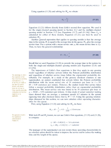
Using equation (11.20) and solving for W q , we obtain:

L q
W q ¼ (11:21)

Equation (11.21) follows directly from Little’s second flow equation. We used it
for the single-channel queuing model in Section 11.2 and the multiple-channel
queuing model in Section 11.3 [see Equations (11.7) and (11.14)]. Once L q is
calculated for either of these models, Equation (11.21) can then be used to
calculate W q .
Another general expression that applies to queuing models is that the average
time in the system, W, is equal to the average time in the queue, W q , plus the average
service time. For a system with a mean service rate , the mean service time is 1/ .
Thus, we have the general relationship:

1
W ¼ W q þ (11:22)

Recall that we used Equation (11.22) to provide the average time in the system for
both the single-and multiple-channel queuing models [see Equations (11.8) and
(11.15)].
The importance of Little’s flow equations is that they apply to any queuing
model regardless of whether arrivals follow the Poisson probability distribution
The advantage of Little’s and regardless of whether service times follow the exponential probability dis-
flow equations is that tribution. For example, in a study of the grocery checkout counters at one
they show how operating
characteristics L, L q , supermarket, an analyst concluded that arrivals follow the Poisson probability
W and W q are related in distribution with the mean arrival rate of 24 customers per hour or l ¼ 24/
any queuing system. 60 ¼ 0.40 customers per minute. However, the analyst found that service times
Arrivals and service follow a normal probability distribution rather than an exponential probability
times do not have to
follow specific probability distribution. The mean service rate was found to be 30 customers per hour or
distributions for the flow ¼ 30/60 ¼ 0.50 customers per minute. A time study of actual customer waiting
equations to be times showed that, on average, a customer spends 4.5 minutes in the system
applicable.
(queuing time plus checkout time); that is, W ¼ 4.5. Using the queuing relation-
ships discussed in this section, we can now calculate other operating character-
istics for this queue.
First, using Equation (11.22) and solving for W q , we have:
1 1
W q ¼ W ¼ 4:5 ¼ 2:5 minutes
0:50
The application of Little’s With both W and W q known, we can use Little’s flow equations, (11.19) and (11.20),
flow equations is to compute:
demonstrated in
Problem 14.
L= W ¼ 0:40ð4:5Þ¼ 1:8 customers
L q ¼ W q ¼ 0:40ð2:5Þ¼ 1 customer

The manager of the supermarket can now review these operating characteristics to
see whether action should be taken to improve the service and to reduce the waiting
time and the length of the queue.

Copyright 2014 Cengage Learning. All Rights Reserved. May not be copied, scanned, or duplicated, in whole or in part. Due to electronic rights, some third party content may be suppressed from the eBook and/or eChapter(s). Editorial review has
deemed that any suppressed content does not materially affect the overall learning experience. Cengage Learning reserves the right to remove additional content at any time if subsequent rights restrictions require it.