Page 618 -

598 CHAPTER 14 MULTICRITERIA DECISIONS

P 1 Problem
Min d þ
1
s:t:
25U þ 50H 80 000 Funds available
þ
0:50U þ 0:25H d þ d ¼ 700 P 1 goal
1
1

þ
3U þ 5H d þ d ¼ 9000 P 2 goal
2 2
þ

þ

U; H; d ; d ; d ; d 0
2
1
1
2
Graphical Solution Procedure
One approach that can The graphical solution procedure for goal programming is similar to that for linear
often be used to solve a programming presented in Chapter 2. The only difference is that the procedure for
difficult problem is to
break the problem into goal programming involves a separate solution for each priority level. Recall that the
two or more smaller or linear programming graphical solution procedure uses a graph to display the values
easier problems. The for the decision variables. Because the decision variables are nonnegative, we con-
linear programming sider only that portion of the graph where U 0 and H 0. Recall also that every
procedure we use to
solve the goal point on the graph is called a solution point.
programming problem is We begin the graphical solution procedure for the Nicolo Investment problem by
based on this approach. identifying all solution points that satisfy the available funds constraint:
25U þ 50H 80 000
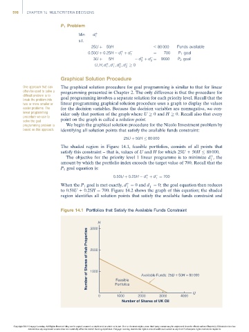
The shaded region in Figure 14.1, feasible portfolios, consists of all points that
satisfy this constraint – that is, values of U and H for which 25U +50H 80 000.
þ
The objective for the priority level 1 linear programme is to minimize d , the
1
amount by which the portfolio index exceeds the target value of 700. Recall that the
P 1 goal equation is:
þ

0:50U þ 0:25H d þ d ¼ 700
1 1
þ

When the P 1 goal is met exactly, d ¼ 0 and d ¼ 0; the goal equation then reduces
1 1
to 0.50U + 0.25H ¼ 700. Figure 14.2 shows the graph of this equation; the shaded
region identifies all solution points that satisfy the available funds constraint and
Figure 14.1 Portfolios that Satisfy the Available Funds Constraint
H
3000
Number of Shares of Hub Properties 2000 Available Funds: 25U + 50H = 80 000

1000
Feasible
Portfolios
U
0 1000 2000 3000 4000
Number of Shares of UK Oil

Copyright 2014 Cengage Learning. All Rights Reserved. May not be copied, scanned, or duplicated, in whole or in part. Due to electronic rights, some third party content may be suppressed from the eBook and/or eChapter(s). Editorial review has
deemed that any suppressed content does not materially affect the overall learning experience. Cengage Learning reserves the right to remove additional content at any time if subsequent rights restrictions require it.