Page 70 -

50 CHAPTER 2 AN INTRODUCTION TO LINEAR PROGRAMMING

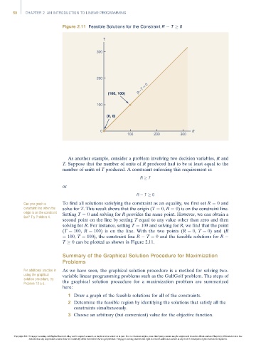
Figure 2.11 Feasible Solutions for the Constraint R T 0

T

300

200
R – T = 0
(100, 100)

100

(0, 0)

0 R
100 200 300

As another example, consider a problem involving two decision variables, R and
T. Suppose that the number of units of R produced had to be at least equal to the
number of units of T produced. A constraint enforcing this requirement is:

R T
or
R T 0

Can you graph a To find all solutions satisfying the constraint as an equality, we first set R ¼ 0 and
constraint line when the solve for T. This result shows that the origin (T ¼ 0, R ¼ 0) is on the constraint line.
origin is on the constraint Setting T ¼ 0 and solving for R provides the same point. However, we can obtain a
line? Try Problem 4.
second point on the line by setting T equal to any value other than zero and then
solving for R. For instance, setting T ¼ 100 and solving for R, we find that the point
(T ¼ 100, R ¼ 100) is on the line. With the two points (R ¼ 0, T ¼ 0) and (R
¼ 100, T ¼ 100), the constraint line R T ¼ 0 and the feasible solutions for R
T 0 can be plotted as shown in Figure 2.11.

Summary of the Graphical Solution Procedure for Maximization
Problems

For additional practise in As we have seen, the graphical solution procedure is a method for solving two-
using the graphical variable linear programming problems such as the GulfGolf problem. The steps of
solution procedure, try
Problem 13 a-d. the graphical solution procedure for a maximization problem are summarized
here:
1 Draw a graph of the feasible solutions for all of the constraints.
2 Determine the feasible region by identifying the solutions that satisfy all the
constraints simultaneously.
3 Choose an arbitrary (but convenient) value for the objective function.

Copyright 2014 Cengage Learning. All Rights Reserved. May not be copied, scanned, or duplicated, in whole or in part. Due to electronic rights, some third party content may be suppressed from the eBook and/or eChapter(s). Editorial review has
deemed that any suppressed content does not materially affect the overall learning experience. Cengage Learning reserves the right to remove additional content at any time if subsequent rights restrictions require it.