Page 67 -

GRAPHICAL SOLUTION PROCEDURE 47

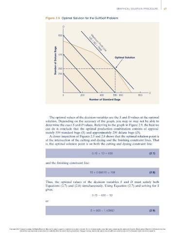
Figure 2.9 Optimal Solution for the GulfGolf Problem

D

600 10S + 9D = 7668

Number of Deluxe Bags 400 Optimal Solution
Maximum Profit Line

250
200

S
0 200 400 550 600 800
Number of Standard Bags

The optimal values of the decision variables are the S and D values at the optimal
solution. Depending on the accuracy of the graph, you may or may not be able to
determine the exact S and D values. Referring to the graph in Figure 2.9, the best we
can do is conclude that the optimal production combination consists of approxi-
mately 550 standard bags (S) and approximately 250 deluxe bags (D).
A closer inspection of Figures 2.5 and 2.8 shows that the optimal solution point is
at the intersection of the cutting and dyeing and the finishing constraint lines. That
is, the optimal solution point is on both the cutting and dyeing constraint line:

0:7S þ 1D ¼ 630 (2:7)

and the finishing constraint line:

1S þ 0:6667D ¼ 708 (2:8)

Thus, the optimal values of the decision variables S and D must satisfy both
Equations (2.7) and (2.8) simultaneously. Using Equation (2.7) and solving for S
gives:
0:7S ¼ 630 1D
or

S ¼ 900 1:4286D (2:9)

Copyright 2014 Cengage Learning. All Rights Reserved. May not be copied, scanned, or duplicated, in whole or in part. Due to electronic rights, some third party content may be suppressed from the eBook and/or eChapter(s). Editorial review has
deemed that any suppressed content does not materially affect the overall learning experience. Cengage Learning reserves the right to remove additional content at any time if subsequent rights restrictions require it.