Page 64 -

44 CHAPTER 2 AN INTRODUCTION TO LINEAR PROGRAMMING

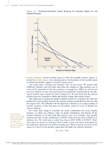
Figure 2.5 Combined-Constraint Graph Showing the Feasible Region for the
GulfGolf Problem

D

1200

1000

Number of Deluxe Bags 800 Sewing

Finishing
600

400

200 Feasible
Region
C & D
I & P
S
0 200 400 600 800 1000 1200 1400
Number of Standard Bags

feasible solutions, and the shaded region is called the feasible solution region, or
simply the feasible region. Any solution point on the boundary of the feasible region
or within the feasible region is a feasible solution point.
Let us just stop a moment and consider what we have done. We started with
GulfGolf’s problem and had little idea what the solution to that problem was in
terms of the quantities of the two products to manufacture. While we still do not
have the solution we have narrowed down the possibilities considerably by identify-
ing the feasible region (shown by itself in Figure 2.6). We now know that the optimal
solution must be somewhere within this feasible region. But exactly where?
One approach to finding the optimal solution would be to calculate the objective
function for each feasible solution; the optimal solution would then be the one with
the largest value. The difficulty with this approach is that there are a huge number of
feasible solutions so this trial-and-error procedure cannot be used to identify the
optimal solution.
So, rather than trying to calculate the profit contribution for every feasible
solution, we select one arbitrary value for profit contribution and identify all the
It’s often useful to
choose an arbitrary value feasible solutions (S, D) that yield this selected value. For example, what feasible
which is a multiple of the solutions provide a profit contribution of $1800? (Note that the value of $1800 is an
two objective function arbitrary one. We could just as easily have chosen $100, $5000 or $2348.97. How-
coefficients (here ever, when we choose an arbitrary value it helps to have one that is convenient for
10 9). This makes
some of the subsequent the arithmetic calculations we will be carrying out.) These solutions are given by the
calculations easier. values of S and D in the feasible region that will make the objective function:
10S þ 9D ¼ 1800

Copyright 2014 Cengage Learning. All Rights Reserved. May not be copied, scanned, or duplicated, in whole or in part. Due to electronic rights, some third party content may be suppressed from the eBook and/or eChapter(s). Editorial review has
deemed that any suppressed content does not materially affect the overall learning experience. Cengage Learning reserves the right to remove additional content at any time if subsequent rights restrictions require it.