Page 46 - Analog and Digital Filter Design

Time and Frequency Response 43

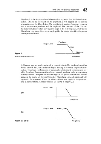
high loss; it is the frequency band where the loss is greater than the desired atten-
uation. Clearly the stopband can be anywhere; it will depend on the desired
attenuation and the filter design. The skirt is the transition frequency response
and is between the passband and the stopband. The steepness of the skirt can
be important; Bessel filters have a gentle slope in the skirt response, while Cauer
filters have very steep skirts. As a rough guide, the steeper the skirt, the poorer
the impulse response.

. Passband

Figure 2.1
Practical Filter Response Frequency

A filter can have a smooth passband, or one with ripple. The stopband can either
have a smooth decay or a series of ripples peaking at a certain stopband atten-
uation. Thus four combinations of passband and stopband responses are pos-
sible. Bessel and Butterworth filters have a smooth passband and a smooth decay
in the stopband. Chebyshev filters have ripple in the passband but have a smooth
decay in the stopband. Inverse Chebyshev filters have a smooth passband with
ripples in the stopband. Cauer (or elliptic) filters have ripple in the passband
and in the stopband. All four variants are shown in Figure 2.2.

Output Level

- L

Frequency

Output Level
+
(b)

Figure 2.2 (a-b) Frequency