Page 123 - Applied Numerical Methods Using MATLAB

112 SYSTEM OF LINEAR EQUATIONS
which can be combined into two formulas as

k−1
u kk = a kk − u 2 ik for k = 1: N (P2.7.3a)
i=1

k−1

u km = a km − u im u ik u kk for m = k + 1: N and k = 1: N
i=1
(P2.7.3b)
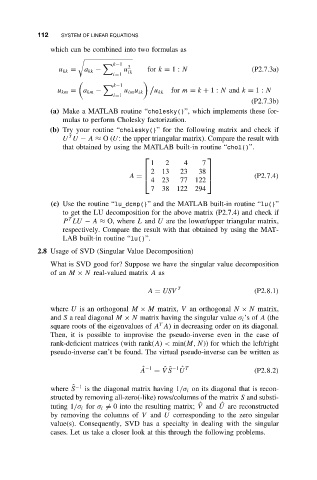
(a) Make a MATLAB routine “cholesky()”, which implements these for-
mulas to perform Cholesky factorization.
(b) Try your routine “cholesky()” for the following matrix and check if
T
U U − A ≈ O(U: the upper triangular matrix). Compare the result with
that obtained by using the MATLAB built-in routine “chol()”.

 
1 2 4 7
 213 23 38 
A =   (P2.7.4)
 4 23 77 122 
7 38 122 294
(c) Use the routine “lu_dcmp()” and the MATLAB built-in routine “lu()”
to get the LU decomposition for the above matrix (P2.7.4) and check if
T
P LU − A ≈ O, where L and U are the lower/upper triangular matrix,
respectively. Compare the result with that obtained by using the MAT-
LAB built-in routine “lu()”.
2.8 Usage of SVD (Singular Value Decomposition)
What is SVD good for? Suppose we have the singular value decomposition
of an M × N real-valued matrix A as

A = USV T (P2.8.1)

where U is an orthogonal M × M matrix, V an orthogonal N × N matrix,
and S a real diagonal M × N matrix having the singular value σ i ’s of A (the
T
square roots of the eigenvalues of A A) in decreasing order on its diagonal.
Then, it is possible to improvise the pseudo-inverse even in the case of
rank-deficient matrices (with rank(A) < min(M, N)) for which the left/right
pseudo-inverse can’t be found. The virtual pseudo-inverse can be written as

ˆ ˆ
A ˆ −1 = V S −1 U ˆ T (P2.8.2)
where S ˆ −1 is the diagonal matrix having 1/σ i on its diagonal that is recon-
structed by removing all-zero(-like) rows/columns of the matrix S and substi-
ˆ
ˆ
tuting 1/σ i for σ i = 0 into the resulting matrix; V and U are reconstructed
by removing the columns of V and U corresponding to the zero singular
value(s). Consequently, SVD has a specialty in dealing with the singular
cases. Let us take a closer look at this through the following problems.