Page 118 - Applied Numerical Methods Using MATLAB

PROBLEMS 107
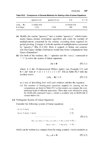
Table P2.3 Comparison of Several Methods for Solving a Set of Linear Equations

gauss(A,b) gaussj(A,b) A\b Aˆ-1*b

||Ax i − b|| 3.1402e-016 8.7419e-016
# of flops 1124 1744 785 7670

(a) Modify the routine “gauss()” into a routine “gaussj()” which imple-
ments Gauss–Jordan elimination algorithm and count the number of
multiplications consumed by the routine, excluding those required for
partial pivoting. Compare it with the number of multiplications consumed
by “gauss()” [Eq. (2.2.18)]. Does it support or betray our expecta-
tion that Gauss–Jordan elimination would take fewer computations than
Gauss elimination?
(b) Use both of the routines, the ‘\’ operator and the ‘inv()’ command or
‘^-1’ to solve the system of linear equations

Ax = b (P2.3.1)

where A is the 10-dimensional Hilbert matrix (see Example 2.3) and
o
o
T
b = Ax with x = [1111111111] . Fill in Table P2.3 with the
residual errors
||Ax i − b|| ≈ 0 (P2.3.2)
as a way of describing how well each solution satisfies the equation.
(cf) The numbers of floating-point operations required for carrying out the
computations are listed in Table P2.3 so that readers can compare the com-
putational loads of different approaches. Those data were obtained by using
the MATLAB command flops(), which is available only in MATLAB of
version below 6.0.

2.4 Tridiagonal System of Linear Equations
Consider the following system of linear equations:

a 11 x 1 + a 12 x 2 = b 1

a 21 x 1 + a 22 x 2 + a 23 x 3 = b 2
···· ··· ···· ··· ··· ···· ··· (P2.4.1)

a N−1,N−2 x N−2 + a N−1,N−1 x N−1 + a N−1,N x N = b N−1
a N,N−1 x N−1 + a N,N x N = b N

which can be written in a compact form by using a matrix–vector notation as
A N×N x = b (P2.4.2)