Page 116 - Applied Numerical Methods Using MATLAB

PROBLEMS 105

%nm2p01.m
.. .. .. .. .. .. .. ..
time_on = 0; time_off = 0;
.. .. .. .. .. .. .. ..
tic
.. .. .. .. .. .. .. ..
time_on = time_on + toc;
tic
xk_off = A\b; %standard LS solution
time_off = time_off + toc;
.. .. .. .. .. .. .. ..
solutions = [x xk_off]
discrepancy = norm(x - xk_off)
times = [time_on time_off]

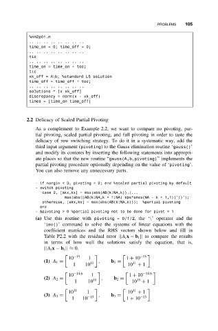
2.2 Delicacy of Scaled Partial Pivoting
As a complement to Example 2.2, we want to compare no pivoting, par-
tial pivoting, scaled partial pivoting, and full pivoting in order to taste the
delicacy of row switching strategy. To do it in a systematic way, add the
third input argument (pivoting) to the Gauss elimination routine ‘gauss()’
and modify its contents by inserting the following statements into appropri-
ate places so that the new routine “gauss(A,b,pivoting)” implements the
partial pivoting procedure optionally depending on the value of ‘pivoting’.
You can also remove any unnecessary parts.

- if nargin < 3, pivoting = 2; end %scaled partial pivoting by default
- switch pivoting
case 2, [akx,kx] = max(abs(AB(k:NA,k))./...
max(abs([AB(k:NA,k + 1:NA) eps*ones(NA-k+ 1,1)]’))’);
otherwise, [akx,kx] = max(abs(AB(k:NA,k))); %partial pivoting
end
- &pivoting > 0 %partial pivoting not to be done for pivot = 1
(a) Use this routine with pivoting = 0/1/2,the ‘\’ operator and the
‘inv()’ command to solve the systems of linear equations with the
coefficient matrices and the RHS vectors shown below and fill in
Table P2.2 with the residual error ||A i x − b i || to compare the results
in terms of how well the solutions satisfy the equation, that is,
||A i x − b i || ≈ 0.
−15 −15
10 1 1 + 10
(1) A 1 = 11 , b 1 = 11
1 10 10 + 1
−14.6 −14.6
10 1 1 + 10
(2) A 2 = 15 , b 2 = 15
1 10 10 + 1
11 11
10 1 10 + 1
(3) A 3 = −15 , b 3 = −15
1 10 1 + 10