Page 113 - Applied Numerical Methods Using MATLAB

102 SYSTEM OF LINEAR EQUATIONS
the Jacobi iteration may be better in speed even with more iterations, since it can
exploit the advantage of simultaneous parallel computation.
Note that the Jacobi/Gauss–Seidel iterative scheme seems unattractive and
even unreasonable if we are given a standard form of linear equations as

Ax = b
because the computational overhead for converting it into the form of Eq. (2.5.3)
may be excessive. But, it is not always the case, especially when the equations
are given in the form of Eq. (2.5.3)/(2.5.4). In such a case, we simply repeat
the iterations without having to use such ready-made routines as “jacobi()”or
“gauseid()”. Let us see the following example.

Example 2.4. Jacobi or Gauss–Seidel Iterative Scheme. Suppose the tempera-
◦
◦
ture of a metal rod of length 10 m has been measured to be 0 C and 10 Cat
each end, respectively. Find the temperatures x 1 ,x 2 ,x 3 ,and x 4 at the four points
equally spaced with the interval of 2 m, assuming that the temperature at each
point is the average of the temperatures of both neighboring points.
We can formulate this problem into a system of equations as
x 0 + x 2 x 1 + x 3 x 2 + x 4
x 1 = , x 2 = , x 3 = ,
2 2 2
x 3 + x 5
x 4 = with x 0 = 0and x 5 = 10 (E2.4)
2
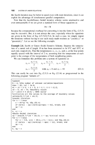
This can easily be cast into Eq. (2.5.3) or Eq. (2.5.4) as programmed in the
following program “nm2e04.m”:

%nm2e04
N = 4; %the number of unknown variables/equations
kmax = 20; tol = 1e-6;
At=[0100;101 0;0101;001 0]/2;
x0 = 0; x5 = 10; %boundary values
b = [x0/2 0 0 x5/2]’; %RHS vector
%initialize all the values to the average of boundary values
xp=ones(N,1)*(x0 + x5)/2;
%Jacobi iteration
for k = 1:kmax
x = At*xp +b; %Eq.(E2.4)
if norm(x - xp)/(norm(xp)+eps) < tol, break; end
xp=x;
end
k, xj = x
%Gauss–Seidel iteration
xp = ones(N,1)*(x0 + x5)/2; x = xp; %initial value
for k = 1:kmax
for n = 1:N, x(n) = At(n,:)*x + b(n); end %Eq.(E2.4)
if norm(x - xp)/(norm(xp) + eps) < tol, break; end
xp=x;
end
k, xg = x