Page 109 - Applied Numerical Methods Using MATLAB

98 SYSTEM OF LINEAR EQUATIONS
(cf) If all the columns of a (complex-valued) matrix A are orthonormal to each other—that
∗T
is, A A = I, or, equivalently, A ∗T = A −1 —it is said to be unitary. It is said to be
−1
T
orthogonal in the case of real-valued matrix with A = A .
SVD (singular value decomposition) is to express an M × N matrix A in the
following form
A = USV T (2.4.14)

where U is an orthogonal (unitary) M × M matrix, V is an orthogonal (uni-
tary) N × N matrix, and S is a real diagonal M × N matrix having the sin-
T
gular values of A (the square roots of the eigenvalues of A A) in decreasing
order on its diagonal. This is implemented by the MATLAB built-in function
svd().

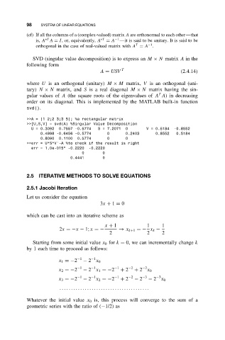
>>A = [1 2;2 3;3 5]; %a rectangular matrix
>>[U,S,V] = svd(A) %Singular Value Decomposition
U = 0.3092 0.7557 -0.5774 S = 7.2071 0 V = 0.5184 -0.8552
0.4998 -0.6456 -0.5774 0 0.2403 0.8552 0.5184
0.8090 0.1100 0.5774 0 0
>>err = U*S*V’-A %to check if the result is right
err = 1.0e-015* -0.2220 -0.2220
0 0
0.4441 0

2.5 ITERATIVE METHODS TO SOLVE EQUATIONS

2.5.1 Jacobi Iteration
Let us consider the equation
3x + 1 = 0

which can be cast into an iterative scheme as

x + 1 1 1
2x =−x − 1; x =− → x k+1 =− x k −
2 2 2
Starting from some initial value x 0 for k = 0, we can incrementally change k
by 1 each time to proceed as follows:

−1
x 1 =−2 −1 − 2 x 0
−2
−1
x 2 =−2 −1 − 2 x 1 =−2 −1 + 2 −2 + 2 x 0
−3
−1
x 3 =−2 −1 − 2 x 2 =−2 −1 + 2 −2 − 2 −3 − 2 x 0
.... ...... ...... ...... ...... ...... .....
Whatever the initial value x 0 is, this process will converge to the sum of a
geometric series with the ratio of (−1/2) as