Page 104 - Applied Numerical Methods Using MATLAB

DECOMPOSITION (FACTORIZATION) 93
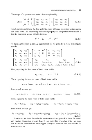
The usage of a permutation matrix is exemplified by

     
001 a 11 a 12 a 13 a 31 a 32 a 33
PA =  100   a 21 a 22 a 23  =  a 11 a 12 a 13  (2.4.2)
010 a 31 a 32 a 33 a 21 a 22 a 23

which denotes switching the first and third rows followed by switching the second
and third rows. An interesting and useful property of the permutation matrix is
that its transpose agrees with its inverse.
T T −1
P P = I, P = P (2.4.3)

To take a close look at the LU decomposition, we consider a 3 × 3 nonsingular
matrix:

     
1 0 0
a 11 a 12 a 13 u 11 u 12 u 13
 a 21 a 22 a 23  =  l 21 1 0   0 u 22 u 23 
a 31 a 32 a 33 l 31 l 32 1 0 0 u 33
   
a 11 a 12 a 13 u 11 u 12 u 13
a 21 a 22 a 23 l 21 u 11 l 21 u 12 + u 22 l 21 u 13 + u 23
  =   (2.4.4)
a 31 a 32 a 33 l 31 u 11 l 31 u 12 + l 32 u 22 l 31 u 13 + l 32 u 23 + u 33
First, equating the first rows of both sides yields

u 1n = a 1n , n = 1, 2, 3 (2.4.5a)

Then, equating the second rows of both sides yields

a 21 = l 21 u 11 , a 22 = l 21 u 12 + u 22 ,a 23 = l 21 u 13 + u 23
from which we can get

l 21 = a 21 /u 11 , u 22 = a 21 − l 21 u 12 , u 23 = a 23 − l 21 u 13 (2.4.5b)

Now, equating the third rows of both sides yields

a 31 = l 31 u 11 , a 32 = l 31 u 12 + l 32 u 22 , a 33 = l 31 u 13 + u 32 u 23 + u 33

from which we can get

l 31 = a 31 /u 11 , l 32 = (a 32 − l 31 u 12 )/u 22 , u 33 = (a 33 − l 31 u 13 ) − l 32 u 23
(2.4.5c)
In order to put these formulas in one framework to generalize them for matri-
ces having dimension greater than 3, we split this procedure into two steps
and write the intermediate lower/upper triangular matrices into one matrix for
compactness as