Page 101 - Applied Numerical Methods Using MATLAB

90 SYSTEM OF LINEAR EQUATIONS
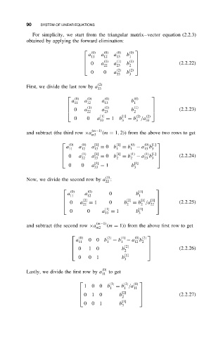
For simplicity, we start from the triangular matrix–vector equation (2.2.3)
obtained by applying the forward elimination:

 (0) (0) (0) (0) 
a a a b
11 12 13 1
 (1) (1) 
 0 a a b (1)  (2.2.22)
22 23
 2 
(2) (2)
0 0 a b
33 3
(2)
First, we divide the last row by a
33
 (0) (0) (0) (0) 
a a a b
11 12 13 1
 (1) (1) (1) 
 0 a a b  (2.2.23)
 22 23 2 
[1] [1] (2) (2)
0 0 a = 1 b = b /a
33 3 3 33
and subtract (the third row ×a (m−1) (m = 1, 2)) from the above two rows to get
m3
 (0) (0) [1] [1] (0) (0) [1] 
a a a = 0 b = b − a b
11 12 13 1 1 13 3
 (1) [1] [1] (1) 
 0 a a = 0 b = b − a b (2.2.24)
(1) [1] 
22 23 2 2 23
 3 
[1] [1]
0 0 a = 1 b
33 3
(1)
Now, we divide the second row by a :
22
 (0) (0) [1] 
a a 0 b
11 12 1
 [2] [2] [1] 
 0 a 22 = 1 0 b 2 = b /a [1]  (2.2.25)
2
 22 
[1] [1]
0 0 a = 1 b
33 3
(m−1)
and subtract (the second row ×a (m = 1)) from the above first row to get
m2
 (0) [2] [1] (0) [2] 
a 00 b = b − a b
11 1 1 12 2
 [2] 
 0 1 0 b  (2.2.26)
2
 
0 0 1 b [1]
3
(0)
Lastly, we divide the first row by a to get
11
 [3] [2] (0) 
1 0 0 b = b /a
1 1 11
 [2] 
 0 1 0 b 2  (2.2.27)
 
[1]
0 0 1 b
3