Page 97 - Applied Numerical Methods Using MATLAB

86 SYSTEM OF LINEAR EQUATIONS
exact solution). If even the RHS element is zero, it should be declared
to be the case of redundancy. In this case, we can get rid of the all-zero
row(s) and then treat the problem as the underdetermined case handled in
Section 2.1.2. If the RHS element is only one nonzero in the row, it should
be declared to be the case of inconsistency.

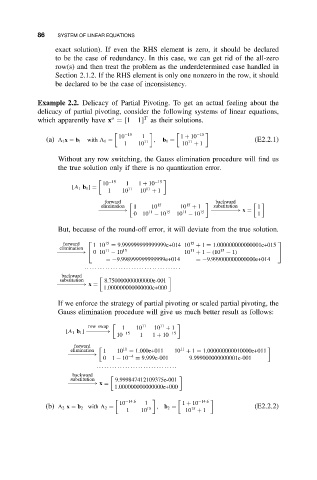
Example 2.2. Delicacy of Partial Pivoting. To get an actual feeling about the
delicacy of partial pivoting, consider the following systems of linear equations,
T
o
which apparently have x = [1 1] as their solutions.
−15 −15
10 1 1 + 10
(a) A 1 x = b 1 with A 1 = 11 , b 1 = 11 (E2.2.1)
1 10 10 + 1
Without any row switching, the Gauss elimination procedure will find us
the true solution only if there is no quantization error.
10 1 1 + 10
−15 −15
[A 1 b 1 ] = 11 11
1 10 10 + 1
forward backward
15
elimination 1 10 15 10 + 1 substitution
1
−−−−−−−→ 11 15 11 15 −−−−−−−−→ x =
010 − 10 10 − 10 1
But, because of the round-off error, it will deviate from the true solution.
15
forward  110 15 = 9.999999999999999e+014 10 + 1 = 1.000000000000001e+015 
elimination
11
15
11
−−−−−−−→  010 − 10 15 10 + 1 − (10 − 1) 
=−9.998999999999999e+014 =−9.999000000000000e+014
... ... ... ... ... ... ... ... ... ... ... ... .
backward
substitution 8.750000000000000e-001
−−−−−−−−→ x =
1.000000000000000e+000
If we enforce the strategy of partial pivoting or scaled partial pivoting, the
Gauss elimination procedure will give us much better result as follows:
11
row swap 1 10 11 10 + 1
[A 1 b 1 ] −−−−−−→ −15 −15
10 1 1 + 10
forward
11
elimination 1 10 11 = 1.000e+011 10 + 1 = 1.000000000010000e+011
−−−−−−−→ −4
0 1 − 10 = 9.999e-001 9.999000000000001e-001
... ... ... ... ... ... ... ... ... ... .
backward
substitution 9.999847412109375e-001
−−−−−−−−→ x =
1.000000000000000e+000
−14.6 −14.6
10 1 1 + 10
(b) A 2 x = b 2 with A 2 = 15 , b 2 = 15 (E2.2.2)
1 10 10 + 1