Page 94 - Applied Numerical Methods Using MATLAB

SOLVING A SYSTEM OF LINEAR EQUATIONS 83
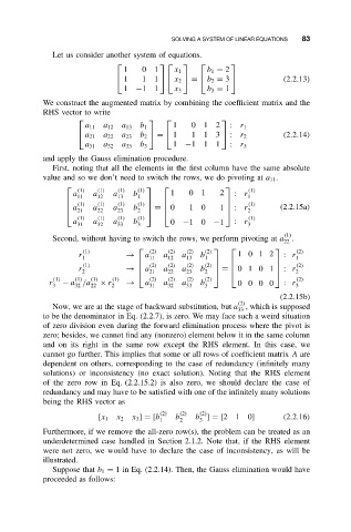
Let us consider another system of equations.
     
1 0 1 x 1 b 1 = 2
1 1 1 = b 2 = 3 (2.2.13)
   x 2   
1 −11 x 3 b 3 = 1
We construct the augmented matrix by combining the coefficient matrix and the
RHS vector to write
   
a 11 a 12 a 13 b 1 1 012 : r 1
 a 21 a 22 a 23 b 2  =  1 113  : r 2 (2.2.14)
a 31 a 32 a 33 b 3 1 −111 : r 3
and apply the Gauss elimination procedure.
First, noting that all the elements in the first column have the same absolute
value and so we don’t need to switch the rows, we do pivoting at a 11 .

 (1) (1) (1) (1)    (1)
a a a b 1 0 1 2 : r
11 12 13 1 1
 (1) (1) (1)    (1)
 a a a b (1)  =  0 1 0 1  : r (2.2.15a)
 21 22 23 2    2
(1) (1) (1) (1) (1)
a a a b 0 −10 −1 : r
31 32 33 3 3
(1)
Second, without having to switch the rows, we perform pivoting at a .
22
(1)  (2) (2) (2) (2)    (2)
r → a a a b 1012 : r
1 11 12 13 1 1

r (1) →  a (2) a (2) a (2) b (2)  =  0101  : r (2)



2  21 22 23 2    2
(1) (1) (1) (1) (2) (2) (2) (2) (2)
r − a /a × r → a a a b 0000 : r
3 32 22 2 31 32 33 3 3
(2.2.15b)
(2)
Now, we are at the stage of backward substitution, but a , which is supposed
33
to be the denominator in Eq. (2.2.7), is zero. We may face such a weird situation
of zero division even during the forward elimination process where the pivot is
zero; besides, we cannot find any (nonzero) element below it in the same column
and on its right in the same row except the RHS element. In this case, we
cannot go further. This implies that some or all rows of coefficient matrix A are
dependent on others, corresponding to the case of redundancy (infinitely many
solutions) or inconsistency (no exact solution). Noting that the RHS element
of the zero row in Eq. (2.2.15.2) is also zero, we should declare the case of
redundancy and may have to be satisfied with one of the infinitely many solutions
being the RHS vector as
(2) (2) (2)
x 3 ] = [b b b ] = [2 1 0] (2.2.16)
[x 1 x 2
1 2 3
Furthermore, if we remove the all-zero row(s), the problem can be treated as an
underdetermined case handled in Section 2.1.2. Note that, if the RHS element
were not zero, we would have to declare the case of inconsistency, as will be
illustrated.
Suppose that b 1 = 1 in Eq. (2.2.14). Then, the Gauss elimination would have
proceeded as follows: